

Study Selection
Participants in this study were recruited from the Osteoarthritis Initiative (OAI), a multicenter, prospective, longitudinal observational study focused on knee osteoarthritis.30Patients with knee arthritis (KL grade ≥1) were selected from the baseline dataset to ensure they had undergone semi-quantitative evaluation of knee radiographs, knee MRI and semi-quantitative evaluation of knee MRI. Of note, all participants enrolled in the study had evidence of osteoarthritis with at least small osteophytes identifiable on radiographs. Following an initial pool of 600 subjects fulfilling these criteria, 567 subjects passed a thorough quality check. These subjects were used to build the model and generate the CAM. After screening by radiologists, we then performed a detailed examination and analysis of the CAM region of 421 eligible patients (see below for details).
MR image selection and quality check
For the subsequent study, we selected sagittal intermediate weighted turbo spin echo (SAG-IW-TSE) sequence images of the subjects' knees. This selection was made based on the availability of the imaging mode to capture structural regions associated with knee pain, including BML, synovitis, effusion, and cartilage loss.31,32,33,34After data collection, a comprehensive examination was performed and 33 abnormal images were identified and excluded by applying the quartile method. These abnormalities included misalignment and the presence of foreign bodies in the slices.
A detailed description of the methodology employed in this study is provided in Supplementary Material S1 and is summarized here (Figure 1 ).

Designing and building models. Each class of model contains submodels.
Construction process for Model 1 and Model 2 (including submodels)
In the initial phase of the study, we developed several models to assess knee pain severity. These models were constructed based on semi-quantitative scores obtained from radiographs and MRIs incorporating various knee structural pathologies. An overview of the elements used to construct these models is as follows: Model 1: Semi-quantitative assessment of fixed flexion knee radiographs. Model 2: Semi-quantitative assessment of knee MR images.
Submodels were then constructed based on factors from Model 1 or Model 2 to further evaluate the severity of knee pain. Details of the specific factors used to construct these submodels are as follows: Model 1.1: OARSI knee score. Model 1.2: KL grade in semiquantitative evaluation of fixed flexed knee radiographs. Model 2.1: cartilage loss in semiquantitative evaluation of knee MR images. Model 2.2: bone marrow lesions in semiquantitative evaluation of knee MR images. Model 2.3: meniscal injury in semiquantitative evaluation of knee MR images. Model 2.4: osteophytes in semiquantitative evaluation of knee MR images. Model 2.5: total knee effusion and synovitis in semiquantitative evaluation of knee MR images. (Because effusion in the selected intermediate-weighted MR scans included effusion and synovitis, effusion and synovitis were combined into one category as used in MOAKS). For a detailed description of the factors employed in these models, additional information can be found in Supplementary Material S1 accompanying this study.
In developing Models 1 and 2, and other models derived from these base models, we employed the K-nearest neighbor (KNN) imputation method to handle missing data. To ensure robustness and mitigate the potential effect of data order on the results, we randomized the data order to enhance robustness.
Model 3 and Model 4 Build Process
We then used neural networks to build models 3 and 4 for assessing knee pain severity. The elements used to build these models were: Model 3: MR images of the knee (four sections of SAG-IW-TSE images) and Model 4: MR images of the knee after feature extraction (four sections of SAG-IW-TSE images).
In Model 3, we preprocessed the data using a normalization technique to convert 2D images into 1D vectors. Again, we randomized the data to improve the validity of the results. In Model 4, we generated a dataset using image features extracted from the images (see below) and processed it in the same way as Model 3.
The model constructed
The construction methodology for each data type was consistent. We used grid search to tune hyperparameters and constructed models using five different methods: Random Forest (RF), Support Vector Machine (SVM), Logistic Regression (LR), Decision Tree (DT), and Bayesian. To maintain consistency across models, we split the data into training and test sets (with randomized index) in a consistent ratio of 9:1. Additionally, we employed 10-fold cross-validation for all models. Finally, we selected the best-performing model. This approach ensures that the selected model is reliable in assessing knee pain severity across different subsets of the dataset.
Evaluating results and model performance
The severity of knee pain due to OA was assessed using the Western Ontario and McMaster Universities Osteoarthritis (WOMAC) pain scale, which ranges from 0 to 20. The scale was derived from a multi-item survey assessing pain experienced during various activities. Knee pain was classified into four groups based on the WOMAC pain score: no pain (score = 0), mild pain (0 < score < 4), moderate pain (score ≥ 4), and severe pain (score ≥ 8).13,35,36.
The area under the curve (AUC) of the receiver operating characteristic (ROC) curve was used as an indicator of model performance. When comparing models, we ensured that all other conditions and methods were consistent. High-performing models were generally considered to have strong correlations and be effective in assessing knee pain severity. All models were built using Python 3.9.
The development of CNN
When constructing the neural network model, we incorporated batch normalization and Rectified Linear Unit (ReLU) as the normalization layer and nonlinear function layer, respectively. Max pooling was used as the pooling technique, and the architecture has five convolutional layers and three pooling layers stacked on top of each other. The output from these layers is connected to the output of three fully connected layers. The input is a two-dimensional image, and the output is a vector of the same length as the number of labels representing the severity of knee pain. The training process used the AdamW optimizer and cross-entropy loss function. Each iteration involved gradient clearing, model forward propagation, loss function backward propagation, and gradient optimization. The classification accuracy of the training set was recorded at each iteration. In addition, forward propagation was performed on the validation set, and the classification accuracy of the validation set was recorded. If the accuracy rate of the validation set in a particular round exceeded the past accuracy rate, the model was saved in a pkl file. Figure 2 shows a schematic diagram of the CNN.
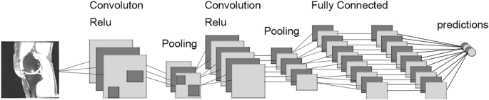
Convolutional Siamese network architecture.
Generating CAM
In our CNN model, global average pooling (GAP) was performed on the final feature map to calculate the average value of each channel, which was then mapped to a class score through a fully connected (FC) layer. The argmax was determined and the gradient of the final feature map was calculated. This gradient was then visualized on the original image to generate the CAM. In this visualization process, the heatmap intensity factor was set to 0.4 to achieve the desired CAM. The CAMs obtained from the four sections of each patient's image were concatenated to present the final result. This approach allows for a comprehensive visualization of the regions in the knee images that significantly contribute to the model's knee pain severity assessment.
A radiologist examines the CAM
A musculoskeletal radiologist with deep expertise in knee MRI interpretation manually reviewed the images and excluded images with insufficient feature extraction or MRI quality. To further streamline the analysis, the radiologist specifically selected subjects whose CAM region was primarily focused on a single lesion within the knee. This targeted selection was to ensure that the analysis was focused on cases where the model's attention was clearly directed to a specific anatomical feature. Statistical analysis was then performed on this refined set of subjects. This approach ensured that the results and conclusions derived from the analysis were based on a subset of subjects on which the model's attention was primarily focused and interpretable.
Informed consent
De-identified data were obtained from the publicly available Osteoarthritis Initiative (OAI) database ( https://oai.nih.gov ), so informed consent was not required.


