Poly R-CNN: Efficient large-scale boundary-regularized building footprint extraction from remote sensing images | Earth Science Informatics

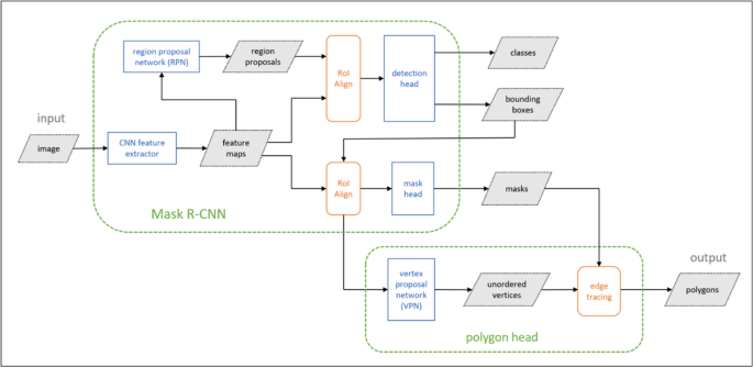
Mask R-CNN is an extension of the Faster R-CNN detection network (Ren et al. 2015), incorporating an additional mask head for image segmentation predictions. Building on this architecture, we further extend the Mask R-CNN model with a polygon head for building polygon predictions, naming it Poly R-CNN. The overall architecture of Poly R-CNN is illustrated in Fig. 1. Unlike most deep learning-based two-stage building extraction methods, Poly R-CNN directly predicts unordered building vertices and then uses a simple post-processing method that leverages the building mask predictions to trace these unordered vertices into polygons. This approach enables Poly R-CNN to avoid the traditional polygon pairing problem during loss computation; instead, it employs the smooth-L1 loss, which has demonstrated remarkable performance in bounding box regression for the Faster R-CNN model, for vertex regression. Additionally, Poly R-CNN takes advantage of the reliable general shape structures of the building masks while avoiding their detailed, twisty boundary shapes. The Vertex Proposal Network (VPN) and edge-tracing components of Poly R-CNN are explained in the following sections.

Vertex proposal network

We propose the VPN, a fast and effective deep neural network that is integrated into Mask R-CNN in parallel with the existing detection and mask heads to directly predict unordered polygon vertices. As shown in Fig. 2, the VPN follows a similar pipeline to the Region Proposal Network (RPN) of Faster R-CNN. It takes the fixed-sized RoIs generated by Mask R-CNN as inputs and generates sets of evenly distributed anchor points on these RoIs. Simultaneously, the RoIs are passed through a 3 × 3 convolutional layer, followed by two 1 × 1 convolutional layers that predict a confidence score and a location offset for each anchor point. These offsets are then decoded using the anchor points to obtain the vertex predictions. Finally, vertex predictions with lower confidence scores within dense clusters are reduced using non-maximum suppression (NMS) to yield the final vertex proposals. The components of the VPN, including anchor point generation, loss design, and NMS, are explained in detail in the following sections.

Anchor point generation

Inspired by the anchor box technique of Faster R-CNN, the VPN uses a method called anchor points to predict polygon vertices. As shown in Fig. 3, anchor points are a set of points evenly distributed across a RoI generated by Mask R-CNN, based on a predefined density value, \(\:d\). For each anchor point, the VPN predicts \(\:x\) and \(\:y\) offsets, along with a confidence score, which represent the displacement of the anchor point from its corresponding object vertex and the model’s confidence that the anchor point aligns with an actual object vertex.

Loss design

Since the VPN is trained to predict a set of x and y regressions and confidence scores for each set of anchor points, target regressions as well as target labels (e.g., foreground/background) for these anchor points are required for training. To generate the target regression values, first, each anchor point is paired with its closest ground-truth vertex. The anchor points that belong to pairs with distances smaller than or equal to a pre-defined threshold f are assigned with a label of 1 (i.e., foreground); the ones that belong to pairs with distances greater than a larger threshold b are assigned with a label of 0 (i.e., background); while the anchor points that belong to pairs with distances between f and b are assigned with a label of -1 (i.e., ignorable). Next, the anchor points and their paired ground-truth vertices are encoded to form the target regressions. The encoding is defined as:

where \(\:{{t}_{x}}^{*}\) and \(\:{{t}_{y}}^{*}\) are the encoded x and y target regression values; \(\:{x}_{gt}\) and \(\:{y}_{gt}\) are the x and y coordinates of the ground-truth vertex; \(\:{x}_{a}\) and \(\:{y}_{a}\) are the x and y coordinates of the anchor point; \(\:{w}_{box}\) and \(\:{h}_{box}\) are the width and height of the predicted bounding box that the anchor points belong to.

To recover the predicted regressions into vertex coordinates, the regression values are decoded using:

where \(\:x\) and \(\:y\) are the decoded vertex coordinates, and \(\:{t}_{x}\) and \(\:{t}_{y}\) are the predicted regression values.

To compare the predicted regressions (\(\:{t}_{x}\) and \(\:{t}_{y}\)) with the target regressions (\(\:{{t}_{x}}^{*}\) and \(\:{{t}_{y}}^{*}\)), we adopt the Smooth-L1 loss:

in which

The L1 loss is preferred over L2 loss in Fast and Faster R-CNN model for bounding box detection. This is because when the regression targets are unbounded, L2 loss can lead to exploding gradients and requires careful tuning of learning rates. L1 loss mitigates this issue by reducing sensitivity to outliers. Since both vertex coordinates (i.e., (x, y)) and bounding box coordinates (i.e., (x_min, y_min, x_max, y^max)) are subject to similar challenges, we also chose L1 loss for vertex prediction.

In addition, the predicted confidence scores are compared with target labels using a binary cross entropy loss:

where \(\:y\) is the target label (i.e., 0 or 1), and \(\:p\) is the predicted probability that the anchor point belongs to a ground-truth vertex.

Non-maximum suppression

The anchor points are regressed toward the ground-truth vertices to form dense clusters of predicted points. To refine these predictions, we apply a simple NMS strategy to retain the point with the highest confidence within each cluster while eliminating the surrounding points. The NMS procedure is as follows:

1. 1)

   Select the predicted point with the highest confidence score (e.g., point \(\:P\)).

2. 2)

   Eliminate all other predicted points within a distance of \(\:l\) pixels from point \(\:P\).

3. 3)

   Retain point \(\:P\) as one of the final vertex proposals and remove it from the list of predicted points.

4. 4)

   Repeat the first three steps until the list of predicted points is empty.

This NMS strategy effectively removes unnecessary or potentially harmful predicted points, resulting in clean, high-quality vertex proposals.

The edge tracing algorithm

Since the VPN predicts unordered vertices, the sequential order of these vertices must be established to form building polygons. To address this, we propose an edge tracing algorithm. First, the algorithm eliminates any extra vertex proposals while determining the sequential order of the selected true vertices. Next, the traced polygons are refined using a corner-sharpening and line-straightening strategy. The steps for vertex tracing and polygon refinement are detailed in Fig. 4.

Vertex tracing

Although the object masks predicted by Mask R-CNN often contain mispredicted pixels along the boundaries, they have demonstrated reliable performance in modeling the general shape structures of objects across various applications. Therefore, we leverage the shape structures of these mask predictions to eliminate unnecessary and imprecise vertices predicted by the VPN while sequentially connecting the true vertices.

First, the boundary coordinates of the pixel-wise binary masks are extracted in a counter-clockwise orientation using the binary image border extraction method described by Suzuki (1985) (i.e., the FindContours function in the OpenCV library). Next, for each mask boundary coordinate, a one-to-one correspondence is established by finding its nearest vertex proposal. Vertex proposals with correspondence distances less than \(\:t\) pixel lengths are selected as the true object vertices. These true object vertices form enclosed polygons by following the same sequential order as the mask vertices. Finally, to avoid redundancy, any consecutively duplicated vertices in the polygons are removed.

Polygon refinement

To ensure highly consistent polygon regularity, we propose a polygon refinement method consisting of two main components: corner sharpening and edge straightening.

Corner sharpening corrects misplaced or missing corner vertices by leveraging prior geometric knowledge of building footprints and the predicted building masks. First, since most real-life building footprints have right-angled corners and edges aligned in two perpendicular directions, we use this prior knowledge to identify two principal directions for each building polygon. The first principal direction is obtained by finding the direction (i.e., rounded to the nearest integer degree, between \(\:[0^\circ\:,180^\circ\:)\) in the polar coordinate system) with the largest sum of edge lengths, while the second principal direction is simply the direction that is perpendicular to the first one and that is also in range \(\:[0^\circ\:,180^\circ\:)\). Next, for each polygon edge \(\:AB\) that belongs to neither of the two principal directions, an additional vertex \(\:C\) is constructed between vertices \(\:A\) and \(\:B\) such that the edges \(\:AC\) and \(\:BC\) belong to the two principal directions. As illustrated by an example shown in Fig. 5, the edge \(\:AB\) does not belong to the determined principal directions of the polygon. Therefore, following the principal directions, two vertex candidates (i.e., \(\:{C}_{1}\) and \(\:{C}_{2}\)) can be constructed between \(\:A\) and \(\:B\). The vertex candinate that has a shorter distance to the nearest mask boundary coordinate is chosen as the vertex \(\:C\) (i.e., \(\:{C}_{1}\)).

For edges with slopes that are approximately aligned with the principal directions, corner sharpening can result in mini-length edges which harms the simplicities and aesthetics of the final polygons. Thus, we propose a line straightening method that eliminates the edges that are shorter than \(\:z\) pixel length. For example, assume \(\:A\), \(\:B\), \(\:C\), and \(\:D\) are four consecutive vertices on a corner-sharpened polygon where the length of edge \(\:BC\) is shorter than the threshold \(\:z\). First, the line straightening method determines which of the edges \(\:AB\) and \(\:CD\) has farther distance to the predicted mask. We define the distance between a polygon edge and a set of mask boundary coordinates as the average distance between a sequence of consecutive mask boundary coordinates and their corresponding projection points on the edge, for which, among all possible sequences of consecutive mask boundary coordinates that can be projected onto the edge, the sequence with the shortest average projection distance is used for the calculation. If an edge cannot be projected by any mask coordinates, the distance between the edge and the mask is considered to be ∞; if both \(\:AB\) and \(\:CD\) have the same distance to the mask, the one with shorter length is considered to be farther. Assuming the edge \(\:AB\) has farther distance to the mask. Then, the vertices \(\:C\) and \(\:D\) are replaced by the projection point of vertex \(\:A\) (i.e., \(\:\:{A}^{{\prime\:}}\)) onto the line extended upon the edge \(\:CD\), such that \(\:A\), \(\:{A}^{{\prime\:}}\), and \(\:D\) forms the new consective vertices. Examples of five major cases of such polyline transformation (i.e., \(\:ABCD\to\:A{A}^{{\prime\:}}D\)) is shown in Fig. 6. For some cases (e.g., Fig. 6(a), (b), (c) and (d)), the transformation results in the vertex \(\:A\) to have an interior angle of 0\(\:^\circ\:\) or 180\(\:^\circ\:\). Therefore, the last step of the line straightening method checks for and eliminates all of such redundant vertices within the polygon. The line straightening method largely reduces the redundancdies of building polygons while preserves their original shape structures.