Less can be more for predicting properties with large language models

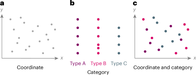
Modeling coordinate information with transformers

Benchmarking with real-world systems can be confounded by inherent correlations within the training data. For example, certain compositions might predominantly form specific structural motifs or crystallize in particular space groups in materials. A model could leverage these statistical correlations to predict a structure-dependent property accurately, even with a limited understanding of the actual geometric arrangements, by primarily relying on compositional cues. To illustrate, if a specific elemental combination almost exclusively forms a known ground state structure, a model might appear to ‘understand’ the geometry leading to this ground state by simply recognizing the composition. This makes it challenging to isolate and quantify a model’s proficiency in processing coordinate information. To address this, we designed hypothetical potentials, where the ‘ground truth’ target values can be continuously tuned to depend more or less on categorical versus positional features. This allows for a systematic probing of a model’s learning capabilities across this spectrum.

The physics-inspired hypothetical potential

We consider a system characterized by a collection of N entities, where each entity k possesses a category type (for example, discrete type) and a continuous coordinate attribute r_k (for example, position). We then define a scalar target value, E, analogous to an energy, for each system configuration. This label is a linear interpolation between a purely category term (E_category) and a purely coordinate term (E_coordinate), controlled by a mixing parameter α ∈ [0,1]

The contribution from category related information, E_category, is defined as a sum over the counts of each entity type

where N_t is the number of unique entity types, n_k is the count of entities of type k, and w_k is a weight associated with particles of type k (in our calculations, we map chemical elements to their energy parameters from the Universal Force Field²⁹). This term represents the contribution of the intrinsic properties of each type of particle. The E_category term captures contributions based solely on the ‘what’ and ‘how many’ of the entities.

The contribution of coordinate-related information, E_coordinate, is designed to depend on the vectors and their relative arrangements

where V(∣r_i − r_j∣) represents a pairwise interaction potential (for instance, Lennard–Jones in our experiments) dependent on the distance between entity i and its neighbors j within a defined neighborhood \({\mathscr{ \mathcal N }}(i)\). This term captures contributions on the basis of the ‘where’ and ‘how arranged’ of the entities.

By varying the mixing parameter α ∈ [0,1], we can continuously tune the nature of the generated target values. In one extreme, at α = 0, the target value E becomes solely dependent on coordinate information (E = E_coordinate). Conversely, at the other extreme, α = 1, the target value depends exclusively on category information (E = E_category). Intermediate values of α, such as α = 0.5, yield labels that represent a balanced contribution from both positional and category terms, while other values within the (0, 1) interval enable a spectrum of relative influences between these two components. Before mixing, both E_category and E_coordinate are independently standardized to zero mean and unit variance across the dataset, ensuring that α controls the relative information contribution rather than differences in raw energy scales. This setup, while a simplification of complex real-world interactions, provides a controlled environment to assess how well a model learns from these distinct information modalities.

CC-cliff

To quantify the model’s relative ability to learn from coordinate versus category information, we define two aggregate metrics: the coordinate contribution (L_coord,α) and the category contribution (L_cat,α). These scores quantify the model’s performance drop in regimes dominated by either coordinate or category information, relative to its performance in a balanced scenario (α = 0.5).

The coordinate contribution (L_coord,α) is calculated by summing the losses for α values where coordinate information dominates, and subtracting a baseline derived from the loss at α = 0.5

where α_g = {0, 0.2, 0.4} is the set of α values biased toward coordinate information, and ∣α_g∣ = 3 is the number of points in this set.

Similarly, the category contribution (L_cat,α) is calculated for α values where category information dominates

where α_c = {0.6, 0.8, 1.0} is the set of α values biased toward category information, and ∣α_c∣ = 3.

A higher contribution (for example, a large positive L_coord,α) indicates that the model struggles more in that respective regime (coordinate-dominant for L_coord,α) compared with the balanced α = 0.5 case. Conversely, a score near zero suggests performance comparable to the balanced case for that regime. The CC-cliff is then analyzed by comparing L_coord,α and L_cat,α. For instance, in Fig. 2, L_coord,α and L_cat,α are plotted against each other.

• If L_coord,α ≫ L_cat,α, the model finds it substantially harder to learn from coordinate information than from category information, relative to the α = 0.5 baseline. If L_cat,α ≫ L_coord,α, the converse is true.

• If L_coord,α ≈ L_cat,α, the model exhibits a similar level of difficulty (or ease) in both regimes relative to the baseline.

This quantitative framework, based on systematically varying the nature of the learning task, enables a more nuanced assessment of an LLM’s capabilities beyond performance on a single, fixed task. It specifically probes the model’s ability for processing and integrating different fundamental types of information present in vector-based descriptions of systems.

n-gram comparison and task complexity variation

Given that our task involves predicting target values on the basis of textual inputs, comparing LLM performance to that of n-gram models provides an informative baseline.¹⁷ Intuitively, n-gram models are not expected to capture complex, nonlocal geometric dependencies or perform intricate calculations (such as those in equation (4)) without an exponentially large number of samples to cover the combinatorial space of token sequences representing these structures. For instance, to accurately model pairwise interactions using only local n-grams, a purely compositional vocabulary might contain around 128 tokens (for elements and digits). However, to also encode atomic positions with a modest 0.1 Å resolution across a 20 Å cell, each atom’s position adds 8 million (8 × 10⁶) possible location identifiers. This inflates the vocabulary of ‘atom-at-a-position’ tokens to over a billion (>10⁹). Learning a simple pairwise interaction (a 2-gram) would require sampling from a space of possibilities that is \({(8\times 1{0}^{6})}^{2}\approx 6.4\times 1{0}^{13}\) times larger than in the compositional-only case. Learning physical laws this way is thus exceptionally sample-inefficient, as it would require an astronomical amount of data to observe a meaningful fraction of relevant atomic pairings.

If LLMs show similar performance trends to n-gram models on this task, it might suggest they are relying on more superficial textual patterns rather than developing a deeper, generalizable understanding of the underlying relationships.

Concurrently, we investigate how the models’ learning capabilities are affected by the ‘resolution of the geometric information’. The calculation of target values, even in our simplified potential (equation (2)), involves operations on continuous vector attributes, such as the pairwise distances ∣r_i − r_j∣ used in E_coordinate. These operations might not align perfectly with a transformer’s natural computational style (cf. RASP conjecture¹⁸), potentially leading the model to learn shortcuts or struggle with precise generalization, especially when the input data (for example, textual representation of crystal structures) requires complex parsing algorithms to extract these from representations of varying length.

Task complexity variation via pairwise distance binning

To probe this, we modify the generation of the target labels E(α) by discretizing the pairwise distances ∣r_i − r_j∣ into a varying number of bins (M) before they are used to calculate E_coordinate (equation (4)). This effectively changes the ‘physical’ model whose properties the LLM must learn:

• When M is small (coarse distance binning), the E_coordinate term, and consequently E(α), is derived from a simplified geometric landscape where only gross differences in inter-entity distances matter. The learning task involves predicting target values from a system with inherently lower geometric resolution.

• When M is large (fine distance binning), E_coordinate and E(α) are derived from a system that is sensitive to subtle variations in distances, more closely approximating a potential based on continuous geometric inputs.

This allows us to assess whether the models are capable of learning fine-grained geometric dependencies when the target values are sensitive to them, or if their performance degrades, potentially indicating an inability to extract or utilize high-resolution continuous information from the textual input, or an over-reliance on coarser patterns. This approach helps to distinguish between a model’s ability to learn a complex function versus its ability to learn a function defined by high-resolution input features.

n-gram model implementation

For the n-gram model experiments, the input system descriptions (for example, CIF files), similar to that used for the LLMs, were used to generate features. Specifically, we extracted term frequency–inverse document frequency³⁰ weighted features from unigrams and bigrams derived from this textual data. An XGBoost³¹ classifier was then trained on these term frequency–inverse document frequency features. The target for these n-gram models was the energy target values, consistent with the task given to the LLMs in the binned experiments described above. The model performance was evaluated using standard classification metrics appropriate for the multi-class problem.

MatText Python package

While tools such as Robocrystallographer ³² and MOFid³³ exist for specific purposes, no unified framework has been available to systematically derive and benchmark multiple text representations across a broad range of crystalline materials. MatText provides an object-oriented way to convert crystal structures into text representations. Each of the text representations has different information content (going from just composition information to information about the composition and the position of all the atoms) (Fig. 4), allowing us to analyze what information language models can use for material property predictions. In addition, the representations feature different combinations of inductive biases, thereby enabling us to identify the most meaningful ones in our analysis. For analysis purposes in this Article, we have categorized representations into broadly three categories: composition-based representations (composition, atom sequence and atom sequence++), representations that focus on local geometry (SLICES and Local-Env) and representations that capture 3D geometry (CIF P₁, CIF Symmetrized, Z-Matrix and Crystal-Text-LLM). More details about inductive biases and various representations with examples are provided in Supplementary Sections 1.2 and 2, respectively.

Scaling experiments

To systematically investigate the impact of scale on performance, we conducted experiments along two primary axes: dataset size and model parameter count. First, we explored data scaling by pretraining BERT models from scratch on datasets of progressively larger sizes. Second, we examined model scaling by applying parameter-efficient fine-tuning to pre-existing Llama-2 models of different scales. The specific setups for these two experimental tracks are detailed below.

Scaling dataset sizes

We created pretraining datasets of four different sizes for all representations shown in Fig. 4. The pretraining datasets are derived from the NOMAD³⁴ database, queried via scripts from MatSciML³⁵ and filtered for 3D crystal structures for which geometry optimization was performed using the PBE functional and the VASP code. Duplicate structures were removed on the basis of CIF symmetry. From the resulting pool of ~2 × 10⁶ unique structures, we randomly sampled subsets of 3 × 10⁴, 1 × 10⁵, 3 × 10⁵ and 2 × 10⁶ structures. For each subset, all nine text representations were derived using the MatText framework, yielding 36 pretraining datasets in total.

We pretrained a separate base BERT model for all these datasets, yielding 36 base BERT models, which were then fine-tuned on different properties from matminer³⁶ (particularly on formation energy of perovskite structures³⁷, bulk modulus³⁸ and shear modulus³⁸, enabling us to compare with state-of-the-art models in MatBench).

Scaling model size

To assess the influence of model scale, we performed parameter-efficient fine-tuning of LLMs of different sizes, specifically, Llama-2 7B, Llama-2 13B and Llama-2 70B models.³⁹ We fine-tune the LLM models with low-rank adaptation (LoRA)⁴⁰. Packing was disabled, and prompt tokens were masked in the loss so that only completion tokens contribute to training. In addition to LoRA, we use 4-bit quantization with nf4 quantization type and float16 compute data type.⁴¹

Hyperparameters

Pretraining

We chose a batch size and context length specific to each representation (given in Supplementary Table 2) and trained for a total of 50 epochs with a learning rate of 2 × 10⁻⁴, using a masked language modeling approach, with a masking probability of 0.15.

Fine-tuning

For fine-tuning, we employ early stopping with a patience of 10 and a threshold of 0.001 to prevent overfitting, utilizing 20% of the data for evaluation while the remaining 80% is used for training. The learning rate is set to 2 × 10⁻⁴. The pretrained base model layers are not frozen, and a regressor head on top of the base model is used for the regression where the embedding of the first token ([CLS] token) is used as the feature for BERT models. All fine-tuning and evaluation were done in a fivefold cross-validation setting.

Following related work^13,42 for Llama fine-tuning, we employed a rank-size of 32 and α_LoRA = 64, with a batch size of eight for 5 epochs and a cosine-annealed learning rate, with no bias applied on a CAUSAL_LM task. We accumulated gradients over four steps and employed gradient checkpointing. The learning rate was set to 3 × 10⁻⁴ with a cosine scheduler, a warm-up ratio of 0.03 and a weight decay of 0.001. Optimization was performed using the paged_adamw_32bit optimizer. A maximum gradient norm of 0.3 was maintained to ensure stable fine-tuning.

Owing to computational limitations, a comprehensive hyperparameter optimization was infeasible. However, for the Llama fine-tuning, we performed some experimentation with the LoRA rank, learning rate and warm-up ratio. We found no meaningful performance difference for rank and learning rate (with results falling within the fivefold cross-validation error bars). The warm-up ratio, however, was more sensitive, as smaller warm-up steps resulted in more invalid generations. All hyperparameter initial values were informed by those calculations^13,42, and we observed no trends that suggest that different parameters would alter the effects seen in the experiments.