physicochemical variables and Acinetobacter The densities of water bodies are shown in Table 1. The mean pH, EC, TDS, and SAL of the water body were 7.76 ± 0.02, 218.66 ± 4.76 μS/cm, 110.53 ± 2.36 mg/L, and 0.10 ± 0.00 PSU, respectively. Mean TEMP, TSS, TBS and DO in the stream were 17.29 ± 0.21 °C, 80.17 ± 5.09 mg/L, 87.51 ± 5.41 NTU and 8.82 ± 0.04 mg/L, respectively, while the corresponding DO5, BOD and AD were They were 4.82 ± 0.11 mg/L, 4.00 ± 0.10 mg/L, and 3.19 ± 0.03 log CFU/100 mL, respectively.
Bivariate correlations between paired PVs varied widely from very weak to complete/very strong positive or negative correlations (Table 2). Similarly, the correlation between various PVs and ADs also changes. For example, there is a very weak but negligible positive correlation between AD and pH (r = 0.03, p = 0.422) and SAL (r = 0.06, p = 0.184), and between AD and TDS. has a very weak inverse (negative) correlation (r = − 0.05, p = 0.243) and EC (r = − 0.04, p = 0.339). There was a significant positive difference between AD and BOD (r = 0.26, p = 4.21E−10), TSS (r = 0.26, p = 1.09E−09), and TBS (r = 0.26, 1.71E−09). A weak correlation is seen. ), on the other hand, AD showed a weak inverse correlation with DO5 (r = −0.39, p = 1.31E−21). There was a moderate positive correlation between TEMP and AD (r = 0.43, p = 3.19E−26), while a moderate negative correlation occurred between AD and DO (r = − 0.46, 1.26E-29).
Explaining contribution of model-predicted AD and PV
The predicted ADs from the 18 ML regression models differ in both mean and coverage (range), as shown in Figure 1. Mean predicted AD ranged from 0.0056 log units by M5P to 3.2112 log units by SVR.Mean AD prediction drops from SVR [3.2112 (1.4646–4.4399)]DTR [3.1842 (2.2312–4.3036)]ENRs [3.1842 (2.1233–4.8208)]NNTs [3.1836 (1.1399–4.2936)]BRT [3.1833 (1.6890–4.3103)]RF [3.1795 (1.3563–4.4514)]XGB [3.1792 (1.1040–4.5828)],Mars [3.1790 (1.1901–4.5000)]LR [3.1786 (2.1895–4.7951)]LRSS [3.1786 (2.1622–4.7911)]GBM [3.1738 (1.4328–4.3036)]Cubist [3.1736 (1.1012–4.5300)]Elm [3.1714 (2.2236–4.9017)]KNN [3.1657 (1.4988–4.5001)]ANET6 [0.6077 (0.0419–1.1504)]ANET33 [0.6077 (0.0950–0.8568)]ANET42 [0.6077 (0.0692–0.8568)]M5P [0.0056 (− 0.6024–0.6916)]. However, regarding the range range XGB [3.1792 (1.1040–4.5828)] and cubism [3.1736 (1.1012–4.5300)] These models outperformed the others because they overestimated AD at lower values and underestimated it at higher values, respectively, when compared to the raw data. [3.1865 (1–4.5611)].

Comparison of AD in water bodies predicted by the ML model. Living Raw/empirical AD values.
Figure 2 presents the explanatory contribution of PV to AD prediction by the model. The subplot AR shows the absolute magnitude (representing parameter importance) by which the PV instances change the AD predictions by each model from the mean value shown on the vertical axis. In LR, absolute changes from mean pH, BOD, TSS, DO, SAL, and TEMP corresponded to absolute changes of 0.143, 0.108, 0.069, 0.0045, 0.04, and 0.004 units in AD predicted responses/values in LR. Did. . Absolute response fluxes of 0.135, 0.116, 0.069, 0.057, 0.043 and 0.0001 in AD predictions were also attributed to pH, BOD, TSS and DO. SAL and TEMP are each dependent on LRSS. Similarly, the absolute changes of DO, BOD, TEMP, TSS, pH and SAL reach 0.155, 0.061. 0.099, 0.144, 0.297 AD prediction response change by KNN. Furthermore, the most contributory or significant PV whose change significantly affected the AD predictive response was RF TEMP (decrease or reduce response up to 0.218). In summary, changes in AD-predicted responses were highest, BOD (0.209), pH (0.332), TSS (0.265), TEMP (0.6), TSS (0.233), SAL (0.198), BOD (0.127), BOD (XGB , BTR, NNT, DTR, SVR, M5P, ENR, ANET33, ANNET64, ANNET6, ELM 0.11), DO (0.028), pH (0.114), pH (0.14), SAL (0.91), and pH (0.427), MARS, Cubist.

PV-specific contributions to 18 ML models predicting AD performance in MHWE receiving water bodies. Mean baseline values of ML PV are displayed on the y-axis. Green/red bars represent the absolute value of each PV contribution in predicting AD.
Table 4 shows the performance of 18 regression algorithms for predicting AD given water PV. Regarding MSE, RMSE, R2XGB (MSE = 0.0059, RMSE = 0.0770; R2= 0.9912) and Cubist (MSE = 0.0117, RMSE = 0.1081, R)2= 0.9827) ranked first and second, respectively, and outperformed the other models in predicting AD. MSE and RMSE metrics include Anet6 (Mse = 0.0172, RMSE = 0.1310), ANRT42 (MSE = 0.0220, RMSE = 0.1483), Anet33 (MSE = 0.0253, RMSE = 0.1590), M5P (M5P = 0.0275, RMSE = 0.16) Ranked. 57), RF (MSE = 0.0282, RMSE = 0.1679) is AD, M5P (R2= 0.9589 and RF (R2= 0.9584) scored better performance on the R-squared metric among the five models, and ANET6 (MAD = 0.0856) and M5P (MAD = 0.0863) on the MAD metric. However, the MAD metric is Cubist (MAD = 0.0437) XGB (MAD = 0.0440).
The importance of each PV feature to permutation resampling on the predictive ability of the ML model in predicting Alzheimer’s disease in water is shown in Table 3 and Figure S1. The ranking of the key variables identified varied by model, with temperature ranking first in 10/18 models. For the 10 algorithms/models, temperature contributed the highest average RMSE dropout loss, with RF, XGB, Cubist, BRT, and NNT temperatures of 0.4222 (45.90%), 0.4588 (43.00%), 0.5294 ( 50.82%). ), 0.3044 (44.87%), and 0.2424 (68.77%), respectively, with RMSE dropouts of 0.1143 (82.31%), 0.1384 (83.30%), 0.1059 (57.00%), 0.4656 (50.58%), and 0.2682 (57.58%). bottom. The losses were attributed to the temperature of ANET42, ANET10, ELM, M5P and DTR respectively. Temperature also ranked second in the 2/18 model, including ANET33 (0.0559, 45.86%) and GBM (0.0793, 21.84%). BOD was another important variable in predicting AD in waters, ranking first in the 3/18 model and second in the 8/18 model. BOD ranked first among important variables in predicting AD for MARS (0.9343, 182.96%), LR (0.0584, 27.42%), GBM (0.0812, 22.35%), but KNN (0.2660, 42.69%) , ranked second in XGB. (0.4119, 38.60); BRT (0.2206, 32.51%), ELM (0.0430, 23.17%), SVR (0.1869, 35.77%), DTR (0.1636, 35.13%), ENR (0.0469, 21.84%), LRSS (0.0669, 31.65%). SAL was ranked first on 2/18 of the models (KNN: 0.2799; ANET33: 0.0633) and second on 3/18 (Cubist: 0.3795; ANET42: 0.0946; ANET10: 0.1359). 2/18 DO 1st (ENR) [0.0562; 26.19%] and LRSS [0.0899; 42.51%]), 2nd on 3/18 (RF [0.3240, 35.23%]M5P [0.3704, 40.23%]LR [0.0584, 27.41%]) model.
Figure 3 shows a residual diagnostic plot of the model comparing the actual AD values to the model-predicted AD values. Observations are LR (A), LRSS (B), KNN (C), BRT 9F), GBM (G), NNT (H), DTR (I), actual AD and predicted AD for SVR showed the value. (J), ENR (L), ANET33 (M), ANER64 (N), ANET6 (O), ELM (P), and MARS (Q) were skewed and smoothed trends did not overlap . However, the actual and predicted AD values are in better agreement, with almost overlapping and smoothed trends seen in RF (D), XGB (E), M5P (K), and Cubist (R). was given. Of the models, both RF (D) and M5P (K) overestimated and underestimated predicted AD at low and high values, respectively. Both XGB and Cubist overestimated AD values at low values, and XGB approached Cubist’s smoothing trend. In general, a smoothed trend that overlaps the slope line is desirable, as it indicates that the model fits all values exactly.
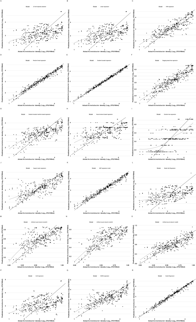
Comparison of actual and predicted ADs by 18 ML models.
For clarity, a comparison of partial dependence profiles of PV in 18-mode AD prediction using the unitary model with PV representation is shown in Fig. 2 and Fig. 3. S2-S7. A partial dependency profile existed for i. A mean increase in AD predictions with increasing PV (uptrend), (ii) a reverse trend in which an increasing PV leads to a decline in AD predictions, and (iii) a horizontal trend in which PV increases and decreases affects AD predictions. (iv) a mixed tendency to switch shapes between two or more of i to iii without giving Model responses varied with changes in PV, especially across breakpoints that could increase or decrease AD predictive responses.
The partial dependence profile (PDP) of DO in the model has a downward trend either from the beginning or after the breakpoints of properties ii and iv, except for ELM, which showed an upward trend (i, Fig. S2). TEMP PDP had an upward trend (i and iv), most often met at one or more breakpoints, whereas LRSS had a horizontal trend (Fig. S3). The PDP of SAL had a typical downward trend (ii and iv) across all models (Fig. S4). LR, LRSS, NNT, ENR and ANN6 showed a typical downward trending PDP for pH, whereas RF, M5P and SVR showed a downward trend filled with various breakpoints. Other models showed typical upward trends (i and iv) filled with breakpoints (Fig. S5). PDP in TSS showed an upward trend returning to a plateau (DTR, ANN33, M5P, GBM, RF, XFB, BRT) after the final breakpoint or decreasing trend (ANNT6, SVR; Figure S6). BOD PDP generally showed an upward trend that was met with breakpoints in most models (Fig. S7).