
Overview of adaptive materials space definition framework
Figure 2 provides an overview of our workflow for operating an autonomous materials exploration system while adaptively redefining the materials space in a data-driven manner. Specifically, we considered an autonomous synthesis platform that can mount three elemental sources and aimed to discover ternary alloys exhibiting a large target property T. The workflow begins with the selection of an initial materials space defined by three randomly chosen metallic elements. Within this space, T is measured for a small number of compositions to obtain initial data.

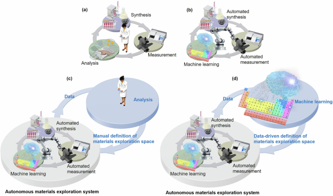
The gray module shows the inner closed-loop autonomous exploration in Fig. 1d (lower left), implementing Bayesian optimization using a Gaussian process regression (GPR) surrogate model and upper confidence bound (UCB) acquisition function. The blue module shows the outer-loop search space redefinition in Fig. 1d (upper right), in which the materials search space is adaptively updated using either the GPR- or large language model (LLM)-based method.
Using these data, the next materials space is redefined in a data-driven manner by selecting a new set of three elements. In this study, the space definition step (shown in blue in Fig. 2) is implemented in two alternative ways: GPR- and LLM-based space definition, as described below. After defining the new space, several compositions within it are randomly sampled, and T is measured to obtain data for autonomous optimization.
Subsequently, autonomous exploration within the newly defined space is performed using a Bayesian optimization framework (shown in gray in Fig. 2). Specifically, a GPR model is constructed with T as the objective variable and the composition vectors as the explanatory variables. Active learning is then performed using the upper confidence bound (UCB) acquisition function39 to identify compositions expected to yield a large T. Once autonomous exploration within the current space is complete, the accumulated data are used again to redefine the subsequent materials space using either GPR or the LLM. By iterating this cycle, the system can execute autonomous exploration while repeatedly and adaptively redefining the materials space in a data-driven fashion. Details of the Bayesian optimization component based on GPR and UCB are provided in the Methods. Below, we describe the GPR- and LLM-based approaches used for adaptive materials space definition.
LLM-driven adaptive materials space definition
The LLM-based approach for defining the next materials space employs an intentionally simple procedure: the LLM is provided with the measured T values and corresponding alloy compositions (formatted as a CSV file), and it is instructed to propose the next materials space by selecting three elements. In this work, we used GPT-5.2 Instant, a generative pre-trained transformer (GPT)-based model developed by OpenAI40. The prompt explicitly constrains the model to avoid reselecting previously explored spaces. In addition to proposing the next combination of three elements, the model is also required to provide a brief rationale for its selection. The prompt and further details are provided in Supplementary Note 1, and sample CSV inputs are provided as Supplementary Data.
GPR-driven adaptive materials space definition
To provide a baseline for comparison with the LLM-based method, a data-driven materials space definition strategy based on a conventional regression model was also implemented. Specifically, a GPR model is trained using the measured T value as the objective variable and composition-based descriptors as the explanatory variables. The descriptors are chemical features generated using the Magpie software package41. The trained GPR model is used to exhaustively predict T for all ternary alloy compositions in the candidate pool. The predicted T values for each three-element combination are then aggregated by computing the mean predicted T over all compositions associated with that combination. The three-element combination with the highest mean predicted value is selected as the next materials space. Details are provided in the Methods section and Supplementary Note 2.
Demonstration
To evaluate the effectiveness of adaptive materials space definition, we conducted a demonstration using a comprehensive dataset derived from high-throughput DFT calculations42. In this demonstration, we focused on composition optimization as a simplified problem setting to illustrate the basic concept and utility of introducing an outer loop for adaptive search space definition. In practical autonomous materials exploration, the search space may also include other variables, such as the crystal structure, synthesis conditions, and processing parameters. Nevertheless, the proposed framework is not intrinsically limited to compositional variables and could, in principle, be applied to broader search spaces by appropriately defining candidate variables and constraints.
The dataset contains the magnetic moment (M), Curie temperature (Tc), and spin polarization (Sp) values of 16,908 ternary alloys with the B2 crystal structure. The magnetic moment M is a fundamental property underpinning applications such as permanent magnets and magnetic devices. The Curie temperature Tc, denoting the transition temperature from ferromagnetic to paramagnetic behavior, is a key metric of the thermal stability of magnetic systems. The spin polarization Sp, defined as the imbalance between up-spin and down-spin electrons at the Fermi level, is critical for spintronic applications, including magnetic sensors and data storage.
Alloys were formed from N = 38 elements: Li, Be, B, Mg, Al, Si, Sc, Ti, V, Cr, Mn, Fe, Co, Ni, Cu, Zn, Ga, Ge, As, Y, Zr, Nb, Mo, Ru, Rh, Pd, Ag, Cd, In, Sn, Sb, Hf, Ta, W, Ir, Pt, Au, and Pb. Because the dataset consists of ternary magnetic alloys, the ferromagnetic elements Fe, Co, and Ni appear relatively frequently, whereas the other elements are more uniformly distributed (Supplementary Note 3). Within each defined materials space, three random measurements were performed, followed by seven iterations of Bayesian optimization using GPR and UCB and definition of the next materials space. This loop was executed for each target property T ∈ {M, Tc, Sp}.
Ten independent runs each of autonomous exploration within spaces adaptively defined by the LLM, GPR, and random selection were performed, for a total of 30 runs. For comparison, ten purely random searches within randomly defined spaces were also conducted. Figure 3a–c shows the evolution of the maximum observed M, Tc, and Sp, respectively, during autonomous exploration. Statistical comparison between the LLM- and GPR-based space definition strategies was performed at observation 25 using two-sided Welch’s t-tests across the ten independent runs.

a–c Evolution of the maximum observed target property (M, Tc, and Sp, respectively) during random and autonomous exploration. The thin red, blue, and green curves are results from ten independent runs using adaptive search space definition by a large language model (LLM), Gaussian process regression (GPR), and random space selection, respectively. The thin black curves are results from ten independent runs of a fully random exploration using randomly selected search spaces. The thick curves denote the mean over ten trials for each strategy.
The LLM-defined workflow (red curves, Fig. 3a) identified high-M materials most rapidly, indicating superior exploration efficiency in the early stage. At observation 25, it showed a nominally significant improvement over the GPR-based strategy (p = 0.0471). This behavior is plausibly attributed to the ability of the LLM to leverage not only the observed M values but also prior knowledge acquired from the literature. Indeed, in the rationale statements accompanying its proposals, the LLM frequently noted that Fe–Co binary alloys are widely known to exhibit large magnetic moments and therefore proposed materials spaces that explicitly include both Fe and Co. In other words, the model appears to possess prior knowledge of the well-established tendency of Fe- and Co-containing alloys to exhibit large M values43. Consequently, it concentrates exploration around such compositions, improving early-stage efficiency.
In contrast, the GPR-based space definition (blue curves, Fig. 3a) relied exclusively on the currently observed M values and associated composition data. Therefore, when the initial randomly chosen space provided limited information about Fe- or Co-containing systems, the model was less likely to propose Fe/Co-rich spaces at the outset. For example, if the initial space consisted of Ni, Al, and Ge, the training set contained only a small number of M measurements for Ni–Al–Ge ternaries, making it unlikely for the GPR-based procedure to consider Fe- or Co-containing spaces as promising at this early stage. Consequently, its early performance was comparable to those of random strategies (green and black curves, Fig. 3a). As exploration proceeded and more data accumulated, the GPR-based method increasingly selected spaces that include Fe and Co, and in the later stage, it became more efficient than random space selection.
The overall trend in Tc (Fig. 3b) mirrored that of M: LLM-based space definition yielded the highest exploration efficiency, consistent with the apparent prior knowledge of the LLM that Fe–Co alloys are well known to exhibit high Tc values43. At observation 25, it exhibited a statistically significant advantage over the GPR-based strategy (p = 0.0216). The GPR-based method again showed limited advantage in the early stage owing to sparse training data but improved with additional observations, eventually outperforming random baselines as it increasingly proposed Fe/Co-containing spaces.
For Sp (Fig. 3c), the LLM-based method showed the highest mean performance, although the difference from that of the GPR-based method was small. Consistent with this trend, the LLM-based strategy did not show a statistically significant advantage over the GPR-based strategy at observation 25 (p = 0.697). This different trend can be plausibly explained by the relative volume of publicly available knowledge: M and Tc are widely studied magnetic properties with abundant accessible information, whereas Sp is comparatively less prominent, potentially limiting the amount of relevant prior knowledge encoded by the LLM. Consistent with this hypothesis, a Google Scholar query performed on 10 February 2026 returned approximately 406,000, 420,000, and 132,000 results for the exact phrases “magnetic moment,” “Curie temperature,” and “spin polarization,” respectively. Thus, the LLM may be able to define spaces more effectively for M and Tc than for Sp for which less information is available.
Selected elements under adaptive materials space definition
To better understand the behavior of space definition strategies, the frequencies with which elements are selected as part of the defined materials spaces were analyzed. Figure 4a and b shows the ten most frequently selected elements under LLM-based space definition in the demonstrations targeting M and Tc. Consistent with the trends in Fig. 3a, b, Fe and Co appeared with the highest frequency, reflecting the prior knowledge of the model that Fe–Co alloys tend to exhibit high M and Tc values.

a–c Large language model (LLM)-based adaptive search space definition. d–f Gaussian process regression (GPR)-based adaptive search space definition.
Figure 4c shows the ten most frequently selected elements under LLM-based space definition for the Sp demonstration, with Co having the highest frequency. Examination of the rationales provided by the LLM suggests a possible correlation between the element selection frequency and knowledge of Co-based Heusler alloys with the L2₁ ordered structure. These alloys are widely known as half-metallic materials (i.e., Sp = 1.0) and have been intensively studied for applications such as magnetoresistive elements and spin-wave devices. Representative examples include Co2MnSi44, Co2MnGe45, Co2CrAl46, Co2FeSi47, and Co2TiGe48. Notably, many of the constituent elements of these alloys were frequently selected by the LLM in our demonstration (Fig. 4c). Furthermore, because the L21 structure can be regarded as B2-like under partial disorder49, this structural relationship may also contribute to the preference of the model for these element combinations.
Figure 4d–f presents the ten most frequently selected elements under GPR-based space definition. The overall trend was qualitatively similar to that for the LLM-based approach, with magnetic elements such as Fe, Co, and Ni selected relatively often. However, these elements appeared less frequently than in the LLM-based case, as the GPR-based strategy relies solely on the observed data and does not leverage prior knowledge from the literature. This difference likely contributes to the lower exploration efficiency of the GPR-based space definition in the early stage.
Another notable global trend was that the LLM-based method frequently selected light elements such as Li and Mg (Fig. 4a–c), whereas the GPR-based method rarely selected them (Fig. 4d–f). The rationales provided by the LLM indicate that Li and Mg were not necessarily selected based on direct evidence that they improve M, Tc, or Sp. Instead, the model appeared to treat them as possible “additive” elements that might modulate material properties through differences in electronic structure and atomic radius relative to transition metals.
To further analyze the origin of early-stage performance differences, the element selection frequencies at the first data-driven space definition step were examined. Figure 5 summarizes the elements appearing in the search spaces at observations 11–20 (i.e., immediately after the first space definition update) for the M, Tc, and Sp demonstrations. Under LLM-based space definition, Fe, Co, and Ni were already selected with high frequency at this early stage (Fig. 5a–c), despite the fact that only limited task-specific training data had been accumulated. This indicates that the LLM recognizes the relevance of these magnetic elements from prior knowledge. By contrast, the GPR-based space definition selected elements more uniformly, without strongly prioritizing magnetic elements (Fig. 5d–f). This is consistent with the fact that this approach infers element importance solely from the small number of early measurements and therefore cannot reliably capture the superiority of Fe/Co-rich spaces at this stage.

a–c Large language model (LLM)-based adaptive space definition. d–f Gaussian process regression (GPR)-based adaptive space definition.
Distribution of autonomously explored materials
To qualitatively compare the exploration behavior induced by LLM- and GPR-based space definitions, the distribution of explored compositions was visualized by t-distributed stochastic neighbor embedding (t-SNE)50. It should be noted that this analysis was intended for qualitative comparison rather than quantitative measurement of compositional diversity. Figure 6a–c shows the two-dimensional embeddings of the 38-dimensional composition vectors of the materials explored in Fig. 3a–c.

a–c Visualization of the 38-dimensional composition vectors explored during autonomous searches targeting the magnetic moment (M), Curie temperature (Tc), and spin polarization (Sp), respectively. The red and blue points denote materials explored using large language model (LLM)- and Gaussian process regression (GPR)-based space definition, respectively. The red arrows highlight clusters enriched in Fe- and Co-containing alloys that emerged during autonomous exploration using the LLM-based space definition.
For the M and Tc demonstrations (Fig. 6a, b), the LLM-based approach produced a dense cluster (indicated by red arrows), suggesting that it repeatedly explored compositionally similar materials. By contrast, the GPR-based approach did not form such a cluster and instead explored more broadly. The clustered region corresponds to alloys containing Fe and Co, consistent with the interpretation that the LLM concentrates exploration around Fe/Co-rich systems based on prior knowledge of their strong magnetic performance. For the Sp demonstration (Fig. 6c), no similarly pronounced cluster was observed, suggesting that the LLM did not focus as strongly on a specific compositional region. This is consistent with the hypothesis that the model possesses less extensive prior knowledge of Sp than M and Tc.

