Determination of disintegration time using formulation data for solid dosage oral formulations via advanced machine learning integrated optimizer models

Data analytics

The dataset of this work has been gathered from a publication which reported data collection for fast-disintegration tablets⁹. This dataset contains around 2,000 entries, with disintegration time as the output and a wide range of input variables which are related to the formulation properties. Input features for building the models in this study include molecular properties of APIs (e.g., hydrogen bonds, molecular weight), composition of tablets excipient (e.g., magnesium stearate, microcrystalline cellulose, chitosan), tablets mechanical characteristics (e.g., friability, hardness), and formulation characteristics (e.g., density, flowability, wetting time) which have been also considered in other studies as inputs for prediction of tablet disintegration times^4,5,8. The same methodology is adopted in this study with different ML models for estimation of DT and compared with other ML models to improve the accuracy of model.

An initial evaluation was carried out on the dataset, and it was turned out that this dataset contains no missing values; therefore, imputation is not required. The subsequent sections of this subsection outline the preprocessing steps applied prior to ML modeling.

Normalization using min-max scaler

In machine learning, data normalization is essential for standardizing feature scales across a dataset. It improves training efficiency and stability, especially for models sensitive to input scale. Without normalization, some features may dominate others, leading to skewed results and reduced model performance.

By employing the Min-Max scaling technique, all values are uniformly scaled in the range 0 to 1. A linear transformation is performed by first subtracting the minimum value of each input and then dividing by its range. The normalization formula using this technique, as shown in Eq. 1, represents this process¹⁰.

This transformation ensures that the values are proportional, making it easier for the model to interpret the data¹¹.

Outlier detection using elliptic envelope

In statistics, the Elliptic Envelope is used to identify anomalies, assuming multivariate normal distributions. In this way, the central distribution and variability of the data points are effectively modeled by defining an elliptical region that captures the majority of samples. Outliers are observations that fall outside of this range¹².

The procedure starts by calculating the mean vector and covariance matrix. Using these statistical estimates, the algorithm constructs an ellipse intended to enclose the core distribution of the data. It is mathematically necessary to optimize the volume of the resulting ellipsoid by ensuring that it contains at least 95% or 99% of the data. The anomalous points are identified as those that are outside the defined elliptical boundary.

Conditional mutual information (CMI)

CMI was used in this study to include the features which identifies the most informative features for regression tasks and fitting the dataset. CMI quantifies the details that one variable conveys regarding the output, conditioned on the presence of a second variable^13,14.

In regression analysis, for \(\:X=[{X}_{1},\dots\:,{X}_{n}]\) as inputs, and \(\:Y\) as outputs, CMI is utilized to quantify the distance or dependency between features as follows^14,15:

CMI, denoted as \(\:I\left({X}_{i};Y|{X}_{j}\right)\), measures the distinct contribution of each feature while considering the effects of other inputs⁸.

TabNet regression model

TabNet is a neural network model tailored for structured datasets, blending strong prediction accuracy with clear model transparency. It utilizes a stepwise attention framework to prioritize important features at each stage, mimicking the logic of decision trees while retaining the adaptability of deep learning methods. This makes TabNet particularly well-suited for predicting disintegration time based on the diverse and complex set of input features in our dataset, including drugs and excipients properties, mechanical properties, excipients composition, and formulation characteristics⁴.

TabNet architecture includes both encoding and decoding modules. The encoder handles input variables by passing them through multiple sequential stages, each containing two main elements: an attention-based selector and a feature transformation unit¹⁶. The feature transformer applies a series of integrated layers and ReLU activations to transform the input features. The attentive transformer generates a sparse mask that determines which features to select for the next decision step¹⁷. This mask is computed using a sparsemax function, which allows for the selection of only the most relevant features while setting others to zero, thereby enhancing interpretability.

Mathematically, the feature selection mask at step (i) is given by:

where, \(\:{P}^{\left[i-1\right]}\) is the prior scale from the previous step, and \(\:{a}^{\left[i\right]}\) is the output of the attentive transformer. The selected features are then used to compute the output of the current step, which contributes to the final prediction.

For the regression task of predicting disintegration time, the outputs from all decision steps are aggregated and passed through a linear layer to produce the final continuous prediction:

where, \(\:{o}^{\left[i\right]}\) is the output from the i-th decision step, and \(\:{W}_{\text{out}}\) and \(\:{b}_{\text{out}}\) are learnable parameters.

The TabNet model is trained to minimize a combination of the mean squared error (MSE) loss for the regression task and a sparsity loss that encourages the model to select fewer features at each step. The sparsity loss is based on the entropy of the feature selection masks and is controlled by a hyperparameter \(\:{\uplambda\:}\). The total loss function is:

RBF-SVR

The Radial Basis Function Support Vector Regression (RBF-SVR) is a robust ML approach used for regression tasks, particularly effective for modeling nonlinear relationships in tabular data. Support Vector Regression (SVR) adapts the core ideas of Support Vector Machines for use in predicting continuous outcomes, aiming to fit a function within a defined epsilon margin around actual values. The Radial Basis Function (RBF) kernel maps input features into a more complex feature space, allowing the model to learn intricate and nonlinear relationships¹⁸.

In this study, the RBF-SVR model is implemented to predict disintegration time based on the input features described above. The model seeks to minimize the error within an epsilon-insensitive tube, where errors smaller than epsilon are ignored, and larger errors are penalized linearly. The RBF kernel is expressed as \(\:K\left({x}_{i},{x}_{j}\right)=\text{exp}\left(-{\upgamma\:}{\left|{x}_{i}-{x}_{j}\right|}^{2}\right)\), where \(\:{\upgamma\:}\) is a kernel parameter controlling the width of the Gaussian function, and \(\:{\left|{x}_{i}-{x}_{j}\right|}^{2}\) is the squared Euclidean distance between two feature vectors \(\:{x}_{i}\) and \(\:{x}_{j}\). Also, SVR optimization problem is formulated as:

subject to:

where w shows the weight vector, b stands for the bias, \(\:{\phi\:}\left({x}_{i}\right)\) maps the input to the higher-dimensional space, C represents the regularization factor balancing margin maximization and error tolerance, \(\epsilon\) is the margin of tolerance, and \(\:{{\upxi\:}}_{i}\), \(\:{{\upxi\:}}_{i}^{*}\) are slack variables for handling errors outside the epsilon tube.

The hyperparameters C, \(\epsilon\), and \(\:{\upgamma\:}\) are critical to the model’s performance and are tuned using cross-validation to optimize predictive accuracy. The training process employs a grid search to identify the optimal combination of these parameters, minimizing the mean squared error (MSE) on the validation set. The final prediction for an input \(\:x\) is given by:

where \(\:{{\upalpha\:}}_{i}\), \(\:{{\upalpha\:}}_{i}^{*}\) are the Lagrange multipliers obtained during optimization. This formulation allows RBF-SVR to effectively model the complex relationships between formulation parameters and disintegration time, providing high predictive accuracy and robustness to outliers, as demonstrated in prior studies.

Neural oblivious decision ensembles (NODE)

NODE model merges the structure of decision trees with the flexibility of neural networks to model tabular data in regression tasks. NODEs are built from a collection of oblivious decision trees, where all data points follow the same split rules at each depth level within a tree, which helps lower variance and improve model stability.

The implementation of the model uses an ensemble of T trees, each with a fixed depth L (e.g., L = 3) and K splits at each level, designed to effectively capture interactions between features. Each node in a tree applies a splitting function \(\:s\left(x;{\uptheta\:}\right)\), parameterized by neural network weights \(\:{\uptheta\:}\), which maps input features x to a binary decision based on a threshold. The splitting function can be expressed as \(\:s\left(x;{\uptheta\:}\right)={\upsigma\:}\left({w}^{T}x+b\right)\), where \(\:{\upsigma\:}\) is a sigmoid activation, w are weights, and b is a bias, determining whether data points move left or right in the tree. The final prediction for an input x is the ensemble average: \(\:\widehat{y}\left(x\right)=\frac{1}{T}{\sum\:}_{t=1}^{T}{f}_{t}\left(x;{{\uptheta\:}}_{t}\right)\), where \(\:{f}_{t}\) is the output of the t-th tree. Training minimizes a MSE loss: \(\:\mathcal{L}=\frac{1}{N}{\sum\:}_{i=1}^{N}{\left({y}_{i}-\widehat{y}\left({x}_{i}\right)\right)}^{2}+{\uplambda\:}{\left|\left|{\uptheta\:}\right|\right|}_{2}^{2}\), using stochastic gradient descent with the Adam optimizer, where \(\:{\uplambda\:}\) stands for a regularization parameter. Hyperparameters T, L, and K are tuned via cross-validation. This mathematical framework ensures NODEs balance interpretability and predictive power, outperforming traditional trees, as shown in prior work¹⁹. The procedure is schematically illustrated in Fig. 1.

Hyper-parameter optimization using WCA

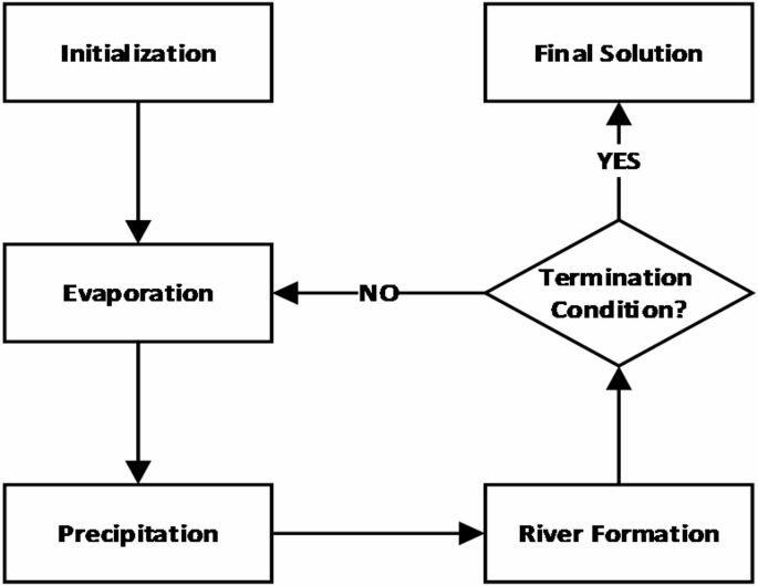
Water Cycle Algorithm (WCA) runs as a metaheuristic optimizer which can be employed for tuning ML hyperparameters. This technique simulates the different stages of the water cycle, such as evaporation, river formation, and precipitation, to investigate optimal solutions^20,21.

In the first phase, a random set of hyper-parameter combinations is generated as potential solutions. In the evaporation phase, solutions are assessed by fitness, with higher values reflecting better performance. These fitness values are crucial in determining the rate of water evaporation^22,23. Water vapor condenses into clouds during the precipitation phase, randomly scattered over the solution set. Every cloud stands for a possible improvement upon a solution. Every cloud’s degree of fitness is assessed; the one with the highest quality is selected²⁴. The identified cloud acts as a reference point for creating a river, directing the existing solution in its direction. This river symbolizes iterative modifications to parameter values. The contrast between the selected cloud and the present solution indicates the necessary updates.

Figure 2 depicts the fundamental sequence of operations in the WCA algorithm. An advantage of this method is its ability to effectively tackle multiple objectives. Multi-objective optimization is a technique that identifies the optimal solutions for goals that are in conflict with each other. The concept is applied to extend WCA optimizer to manage several objectives. If one solution performs better in at least one goal without being less than another, then it is judged to dominate another. Incorporating this idea allows the WCA to find a set of mutually exclusive solutions^21,25.