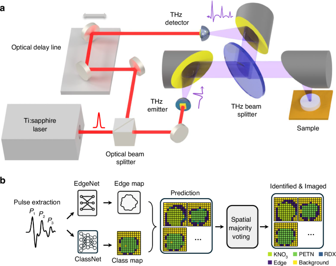
A schematic diagram and the operational principles of the terahertz time-domain spectroscopic imaging system are illustrated in Fig. 1a. The system is driven by a Ti:sapphire laser that generates 135 fs pulses at a central wavelength of 800 nm with a repetition rate of 76 MHz. The laser beam is split into two paths to independently pump and probe the photoconductive terahertz source and detector, both based on plasmonic nanoantenna arrays. Under an applied bias voltage, photo-generated carriers in the active area of the terahertz source drift toward the nanoantenna electrodes, producing sub-picosecond terahertz pulses54. At the detector, photo-generated carriers drift in response to the incident terahertz field, generating a photocurrent proportional to the field strength52. The plasmonic nanoantenna arrays enhance optical absorption near the electrodes through surface plasmon excitation, preserving high quantum efficiency and ultrafast response. This leads to efficient terahertz generation and highly sensitive detection. A mechanical optical delay line in one of the paths introduces a tunable time delay between the pump and probe beams. Terahertz radiation generated at the source is collimated using an off-axis parabolic mirror and then focused onto the sample using a second off-axis parabolic mirror, producing a beam spot with a 2-mm focal size. The sample is positioned on a metallic platform controlled by an XY motorized stage for spatial scanning. The reflected terahertz signal is directed to the detector via a terahertz beam splitter and subsequently focused onto the detector using another off-axis parabolic mirror. The time-domain terahertz electric field at each spatial point of the sample FOV is recorded by measuring the photocurrent from the terahertz detector as a function of the time delay introduced by the optical delay line. Applying a Fourier transform to the time-domain signal yields a broadband power spectrum extending up to 4.5 THz, with a peak dynamic range of 96 dB. This high peak dynamic range enables the robust detection of weak terahertz reflections from irregular and concealed samples in reflection mode. The performance of the system in transmission mode is also evaluated (see Supplementary Fig. S1). Each spectrum is acquired within an integration time of 3 s using pump and probe powers of 600 mW and 150 mW, respectively. The full time-domain response of the sample is obtained by raster scanning the sample FOV and acquiring 10,100 time-domain points at each spatial location.

a Schematic diagram of the terahertz time-domain spectroscopy-based chemical imaging system. The sample is mounted on a metallic stage controlled by a motorized translation stage for raster scanning. b Processing pipeline for chemical classification using terahertz spectral imaging. The workflow incorporates two neural networks: EdgeNet, which identifies sample boundaries/edges, and ClassNet, which performs chemical classification per pixel, generating a class map that preserves the spatial resolution of the edge map. Spatial post-processing in the form of pixel-level majority voting is also applied to enhance the classification accuracy of each chemical image
Using this terahertz spectroscopic imaging system, we analyzed a range of pharmaceutical and explosive materials. The four pharmaceutical compounds—MCC, DCP, MAN, and IBU—were compressed into cylindrical tablets using a hydraulic pellet press. Each tablet had a diameter of 10 mm, with thicknesses ranging from 2 to 4 mm. The four explosives examined—KNO₃, PETN, RDX, and TNT—were not suitable for high-pressure tablet formation due to explosion risk. Instead, they were mounted in an aluminum holder featuring a cylindrical cavity with a 10 mm diameter. The explosive samples placed in the holder had thicknesses between 2 and 4 mm. All samples were raster scanned over a 12 × 12 mm² area with a spatial step size of 1 mm. A 12 × 12 mm² area was scanned in ~447 s. This duration includes a 3-s acquisition time per pixel plus the time needed for stage movements between successive points.
Following data acquisition, the terahertz signals were processed using two dedicated neural networks—which we termed EdgeNet and ClassNet—for chemical identification and classification. Figure 1b illustrates the full data processing pipeline, encompassing the terahertz imaging, neural network inference, and spatial post-processing. First, the system acquires time-domain waveforms corresponding to each chemical sample. These pulses are then extracted and used as inputs to the two neural networks for edge detection and chemical classification.
EdgeNet functions as a binary classifier, distinguishing boundary pixels from non-boundary pixels to identify the presence or absence of edges within the sample FOV. At each pixel location, EdgeNet processes all the extracted terahertz pulses together to make its decisions. In parallel, ClassNet operates on an individual pulse basis, processing each pulse separately to generate probabilistic predictions for the chemical class, including the identification of the background sample holder (metal) if there is no sample for that pixel. For each pixel, these predictions are aggregated using a winner-takes-all strategy, where each pixel is assigned to the class with the highest predicted probability. Finally, the outputs of EdgeNet and ClassNet are integrated through a decision algorithm to determine the final classification of each pixel across the entire sample FOV. To further enhance our image-based classification accuracy, spatial majority voting and morphological operations are applied as post-processing steps (refer to Methods for details). These techniques incorporate local spatial context, helping to suppress inference artifacts and generate cleaner, more accurate chemical images that preserve the true spatial distribution of the material under test.
The distinct input structures for EdgeNet and ClassNet are custom tailored to their specific objectives. EdgeNet leverages the collective information from all the extracted terahertz pulses to make its decisions. This allows the network to identify complex temporal signatures, such as multiple reflections and scattering artifacts, that are characteristic of material boundaries. In contrast, for chemical classification, ClassNet processes each pulse individually, generating probabilistic predictions for the chemical class of each pixel, including the identification of the background sample holder. This approach was designed to preserve the unique spectral features within each reflection that are critical for identifying the chemical type of interest.
When the terahertz beam is focused onto a sample, as illustrated in Fig. 2a, multiple reflected pulses are captured in a single time-domain scan. Typically, four distinct pulses are observed in this reflection-mode setup, denoted as P1, P2, P3, and P4: P1 corresponds to the reflection from the sample’s top surface and contains surface reflectance information; P2 is the reflection from the metal substrate and does not carry chemical information; P3 arises from the sample’s bottom interface and contains key absorption features representative of the material; P4 and subsequent pulses are due to internal multiple reflections and also encode absorption characteristics of the sample under test. For reference, the pulse reflected from the metal background is nearly identical in shape to P2 (see Supplementary Fig. S2). While our analysis focuses on these four primary reflections, a time-domain trace can contain additional pulses. These typically arise from artifacts like edge scattering or from extra layers like a paper cover, which we will detail in subsequent measurements. The relative sequence and timing of these pulses vary depending on how the sample is positioned, and this information is assumed to be unknown to our neural networks.

a Reflected terahertz time-domain response from a KNO₃ sample. When the terahertz beam is incident near the sample edges, at least four distinct reflected pulses are observed. The first pulse (P1) corresponds to the reflection from the sample’s top surface; the second pulse (P2) originates from the metallic background (sample holder); the third pulse (P3) arises from the bottom interface of the sample; and the fourth one (P4) results from an internal reflection following two round trips within the sample. The inset shows the calculated terahertz absorption spectrum of KNO₃, derived from the third and second pulses. b–e Cropped waveforms of the four reflected pulses by pulse extraction algorithm in (a), each with a duration of 13 ps. After performing pulse extraction for every pixel across the 12 mm × 12 mm raster scan area, f–i represent the color maps of the peak amplitude values for each pulse (P1–P4)
While the material’s terahertz absorption spectrum can be obtained by calculating the Fourier transform of P3 relative to the reference pulse P2, as illustrated in the inset of Fig. 2a, directly applying a Fourier transform to the entire time-domain waveform can be unreliable, as interfering pulses may distort the spectral signatures. To mitigate this, we adopt a pulse-based chemical classification strategy. This approach significantly improves the robustness of inference by enabling classification that is insensitive to pulse order or temporal spacing—parameters that can fluctuate with changes in the sample geometry, placement, and packaging. Each full time-domain waveform per pixel is segmented into individual pulses with a duration of 13 ps, each consisting of 650 data points, as illustrated in Fig. 2b–e. The 13-ps time window is sufficient to capture a terahertz pulse and provides a spectral resolution of 76.9 GHz, which is adequate for our classification task. After performing the same pulse extraction for every pixel across the FOV, we take the peak amplitude value for each pulse (P1–P4) at each pixel to construct the 2D maps, as shown in Fig. 2f–i. The peak amplitudes of these pulses exhibit strong spatial correlation and track the geometry of the sample. This peak amplitude data is also central to our automated processing pipeline. For pulse extraction, a global detection threshold is applied to all waveforms to consistently identify potential pulses while rejecting noise. Following pulse extraction, the algorithm performs two labeling tasks to generate the training data. First, it categorizes each pulse—distinguishing between sample and background reflections—by using pulse timing in conjunction with prior knowledge of the sample’s structure (only used for training). Second, we determine a sample-specific amplitude threshold to identify edges; this value is set higher than the initial global detection threshold. Any pixel where the detected pulses fall below this second threshold is labeled as an “edge”, representing the weak scattering signals typical of sample boundaries (see Methods for details). These isolated pulses, without their relative time delay information, are used as individual inputs to a neural network trained to predict the chemical composition at each spatial location. This strategy enhances the system’s resilience to environmental variability and enables reliable, pixel-level chemical identification across diverse real-world scenarios, including concealed chemicals.
Figure 3 illustrates the architectures of the two neural networks used in our chemical imaging and classification pipeline: EdgeNet and ClassNet. EdgeNet (Fig. 3a) is designed for binary edge detection and is implemented using a 4-layer transformer encoder55. It accepts an input tensor of size 8 × 650, where each row corresponds to a distinct terahertz pulse; if less than 8 pulses are available per pixel, zeros are padded for the remaining pulse entries. Self-attention-based feature extraction is applied to extract features across the pulse set56, followed by a mean pooling operation along the sequence dimension. The resulting feature vector is passed through a fully connected layer to generate class probabilities indicating the presence or absence of an edge per pixel within the sample FOV. Notably, we did not incorporate temporal positional encoding, which is commonly used in transformer architectures, as the order of the input pulses may be unknown or not repeatable in real-world scenarios (e.g., for concealed chemicals). This design choice improves the model’s robustness to unknown variations in pulse ordering. The internal structure of the transformer encoder (Fig. 3b) consists of layer normalization, a multi-head self-attention mechanism, and a feedforward multilayer perceptron (MLP), connected through residual pathways to facilitate gradient flow. The multi-head attention module (Fig. 3c) comprises eight parallel attention heads (h = 8), each computing scaled dot-product attention over the input sequence.

a EdgeNet is built on a transformer backbone for edge detection; it outputs the probabilities of 2 classes: Edge/Other. b The internal structure of the transformer encoder, featuring a multi-head self-attention mechanism. c The schematic of a multi-head attention. d ClassNet, implemented using a CNN for multi-class chemical classification. EdgeNet leverages the global contextual modeling capabilities of transformers to accurately detect sample boundaries, while ClassNet utilizes the local feature extraction strengths of CNNs to enable efficient and robust chemical identification within the sample FOV. B: batch size
ClassNet (Fig. 3d), in contrast, is used for multi-class chemical classification at each pixel and is based on a CNN architecture57. It processes individual terahertz pulses through two 1D convolutional layers with ReLU activation and max pooling. The resulting feature maps are flattened and passed through two fully connected layers. A final softmax layer produces the probability distribution over the target chemical classes per pixel. Together, EdgeNet and ClassNet provide complementary capabilities—enabling accurate spatial boundary detection of the sample under test and robust pixel-level chemical classification within our spectroscopic imaging framework.
We trained both ClassNet and EdgeNet using pharmaceutical and explosive samples. To evaluate their generalization capability, the models were tested on entirely new, previously unseen samples and data. Figure 4 summarizes the blind classification results for these chemical test samples. In Fig. 4a, we present representative images of unknown chemical samples alongside the corresponding ground truth labels, model predictions before the spatial majority voting, and refined predictions after applying spatial majority voting for eight material classes: DCP, MCC, IBU, MAN, KNO₃, PETN, RDX, and TNT (see Methods for details). While the raw predictions from the two networks already demonstrated high classification performance, spatial majority voting further improved the results by mitigating spatially isolated pixel-level misclassifications, while also enhancing the edge detection accuracy, correctly revealing the boundaries of chemical objects. The overall pixel-level classification performance of our approach is quantitatively captured in the confusion matrix shown in Fig. 4b, which demonstrates consistent high accuracy across all chemical classes with minimal cross-class confusion. Specifically, the model achieved pixel-level classification accuracies of 99.48%, 98.26%, 100%, 100%, 100%, 100%, 99.57%, and 98.89% for DCP, MCC, IBU, MAN, KNO₃, PETN, RDX, and TNT, respectively. The average accuracy, including the background region (i.e., the sample holder, without a chemical), reached 99.42%. In addition, Fig. 4c demonstrates our model’s strong performance on spatially irregular and cracked test samples, even though it was trained exclusively on intact, regular samples. This successful generalization is rooted in our pulse-based approach. The full time-domain waveforms for intact versus cracked samples differ in pulse timing and relative amplitudes (see Supplementary Fig. S3). However, the characteristic shape of the crucial P3 pulse remains consistent between them. Because our network analyzes individual pulse shapes, it correctly identifies the material despite these structural irregularities. Furthermore, our model demonstrates its generalization capability by accurately predicting four different types of cracked pharmaceutical samples in the same FOV (see Supplementary Fig. S5). These results underscore the robustness of our classification pipeline, highlighting its ability to handle challenging and previously unseen sample conditions.

a Representative input images, ground truth labels, model predictions before spatial majority voting, and refined predictions after spatial majority voting for DCP, MCC, IBU, MAN, KNO₃, PETN, RDX, and TNT. b Confusion matrix summarizing the classification performance across all the chemical classes. c Ground truth and model predictions for cracked, irregularly shaped pharmaceutical samples, demonstrating the models’ ability to generalize to new test samples despite being trained exclusively on intact, regular samples
We further evaluated the performance of our classification pipeline on concealed chemical samples, where the substances were hidden beneath a visibly opaque paper cover and not detectable under standard illumination or visible or IR-based machine vision, as illustrated in Fig. 5. Importantly, the network models were trained exclusively on uncovered samples; thus, this evaluation tests their external generalization capability in realistic scenarios where chemical substances may be obscured within envelopes, packages/bags, or other visually inaccessible environments. Figure 5a shows a schematic of the experimental setup, in which each sample is covered/obscured by paper. Representative ground truth labels and our model predictions (after spatial majority voting) for four hidden explosives—KNO₃, PETN, RDX, and TNT—are shown in Fig. 5b. Despite the paper-based concealment, our models accurately recover the spatial distributions of these chemicals and specifically identify the type of chemicals.

a Schematic illustration of chemical classification through a visibly opaque paper cover; the explosive samples were hidden, i.e., remained undetected under visible illumination. b Ground truth labels and model predictions after spatial majority voting for KNO₃, PETN, RDX, and TNT. c Confusion matrix summarizing the classification performance for the concealed explosive samples. d Sample pictures with and without concealment, and our network predictions for a scenario involving multiple types of concealed chemicals within the same field of view. Note that the models were trained exclusively on uncovered samples
The confusion matrix in Fig. 5c summarizes the classification results, with the model achieving accuracies of 76.20% (KNO₃), 94.42% (PETN), 98.64% (RDX), and 87.90% (TNT). The average accuracy, including the background class, is 88.83%. Additionally, Fig. 5d showcases the model’s performance in a more complex scenario: identifying multiple types of chemicals concealed under a paper cover within the same FOV. While the cover introduces an additional reflection pulse (see Supplementary Fig. S4), the key pulses of interest retain their characteristic shapes after our extraction process. Consequently, the model successfully differentiates between all hidden chemical regions, highlighting its robustness and generalization under challenging and practically relevant imaging conditions.