Advanced predictive modeling for municipal solid waste management using robust machine learning

In order to investigate and compare the performance of different algorithms, several statistical evaluation methods are adopted in this study, as shown in Equations 1 and 2. (1-5). These statistical parameters are chosen because they provide a robust framework for quantitatively evaluating each algorithm’s accuracy, consistency, and predictive ability. Applying these metrics makes it possible to perform systematic comparisons and identify the most effective algorithms for predictive modeling in this area. The use of such parameters ensures objective performance evaluation and supports evidence-based conclusions about the efficiency of the model.

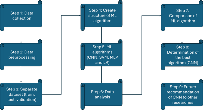
In this study, four advanced machine learning algorithms, namely CNN, SVM, MLP, and LR, were applied to develop a predictive model for effective management of municipal solid waste. The results and performance metrics of these algorithms are comprehensively presented in Tables 4, 5, and 6. Of the 3,000 randomly selected data points, 70% were used for training, 15% for testing, and 15% for validation. This analysis highlights the great potential of artificial intelligence in various aspects of municipal solid waste management, especially in optimizing waste collection processes. By leveraging data-driven insights, these machine learning models contribute to more efficient route planning, timely waste collection, resource allocation, and overall operational efficiency. Moreover, the application of such intelligent systems supports strategic planning and policy development by enabling accurate predictions and real-time monitoring. Ultimately, the integration of artificial intelligence into municipal solid waste management offers an innovative approach that can significantly improve environmental sustainability, reduce operational costs, and promote cleaner and more livable urban environments.

Table 4, Table 5, and Table 6 show the statistical results of MSWM predictive modeling using training, testing, and validation datasets using advanced ML algorithms (CNN, SVM, MLP, and LR). Among them, CNN consistently shows superior prediction accuracy across all evaluation metrics. According to Table 5, CNN yields ARE = ​​-0.96, AARE = ​​2.05, SD = 1.0, RMSE = 1.1, and R² = 0.996, showing better performance than other models. The MLP results are ARE = ​​-3.01, AARE = ​​4.14, SD = 2.47, RMSE = 2.38, and R² = 0.870. SVM shows ARE = ​​0.97, AARE = ​​4.60, SD = 3.94, RMSE = 3.70, and R² = 0.861. LR shows ARE = ​​4.07, AARE = ​​6.81, SD = 5.92, RMSE = 5.21, and R² = 0.853. These findings support the robustness and higher predictive ability of CNN than other applied ML models in estimating MSWM parameters.

Figure 8 shows a crossplot diagram showing the predictive performance of different machine learning algorithms (CNN, SVM, MLP, LR) in estimating MSWM using the test dataset. Each subplot shows a scatterplot in which the predicted values ​​are plotted against the actual values, accompanied by a trend line and its corresponding R.² A value indicating goodness of fit. CNNs exhibit a strong linear relationship between predicted and actual values, as evidenced by a high R.²The value is 0.996, indicating good prediction accuracy. MLP also shows a good fit in R.² The value is 0.870, indicating a reasonable ability to predict MSWM. Similarly, SVM and LR demonstrate comparable predictive capabilities using R.² The values ​​are 0.861 and 0.853, respectively. Although all models show a positive correlation between predicted and actual values, the CNN model clearly outperforms the other models in terms of MSWM prediction accuracy.

Figure 9 shows the statistical parameters of ARE, AARE, and SD for predicting MSWM using the test dataset and robust machine learning algorithms (CNN, MLP, SVM, LR). Each spoke of the radar chart represents one machine learning model, and the lines radiating from the center indicate the magnitude of the statistical parameter. The CNN model shows relatively low values ​​for all 3 error metrics, especially ARE and AARE, suggesting high accuracy and minimal bias in prediction. The MLP and SVM models show comparable error characteristics, with slightly higher values ​​of ARE, AARE, and SD compared to CNN, indicating a moderate level of prediction accuracy. Although the LR model still shows reasonable performance, it shows somewhat higher error values ​​for all three parameters, suggesting lower accuracy and higher prediction dispersion compared to other models. In general, the closer the line is to the center of the radar chart, the better the model performs in terms of smaller MSWM prediction errors and higher accuracy.

Figure 10 is a histogram diagram showing the distribution of prediction errors for MSWM using the test dataset across four robust machine learning algorithms: CNN, SVM, MLP, and LR. Each subplot shows the frequency of errors overlaid with a normal distribution curve. For CNN, the histogram is tightly centered around zero, with a very small mean (0.000001069) and standard deviation (0.0001301), indicating minimal error, low variability, and highly accurate predictions. In contrast, SVM exhibits a broader distribution of errors centered around a mean of -8.562 and a much larger standard deviation of 62.37, suggesting more significant and diverse prediction errors. Similarly, MLP shows errors distributed around a mean of -0.3644 and a standard deviation of 7.047, indicating a moderate level of error and variability. Finally, LR also exhibits a distribution of errors with a mean of -0.4992 and a standard deviation of 6.846, making it comparable in performance to MLP in terms of error magnitude and spread. The visual comparison clearly shows that the CNN model produces the most accurate predictions with the lowest error diffusion among the evaluated algorithms.

Figure 11 shows the error parameter diagram for predicting municipal solid waste management (MSWM) using the test dataset with robust machine learning algorithms (CNN, SVM, MLP, and LR). Each subplot displays the distribution of decision error across the data points. For CNN, the errors are consistently very close to zero and vary within a narrow range (approximately – 0.0004 to 0.0005), indicating high accuracy and stable predictions with minimal deviations. In contrast, SVM shows a wider margin of error, varying between approximately -10 and 15, suggesting that the difference between predicted and actual values ​​is larger and more varied. MLP shows a similar but slightly wider error range, mostly between − 5 and 15, but with occasional larger negative spikes reaching around − 60, indicating some significant subpredictions. LR shows the largest error range and varies significantly between approximately -80 and 60, highlighting its low accuracy and susceptibility to large prediction errors compared to other models. This visual comparison clearly shows the superior performance of the CNN model in terms of error magnitude and consistency of MSWM predictions.

Figure 12 shows a bar graph comparing the statistical parameters of MSE, RMSE, and R.²Predict municipal solid waste management (MSWM) using a test dataset with CNN, MLP, SVM, and LR machine learning algorithms. The CNN model shows good performance with the lowest MSE and RMSE values, indicating the least prediction error and achieving the highest R at the same time.² A value (close to 1.0) indicates a good fit to the data. According to CNN, the MLP model shows moderate MSE and RMSE values ​​and moderately high R.²suggesting good predictive ability. Although the SVM model has lower MSE and RMSE than LR, it still exhibits higher error metrics and lower R.² Compare with CNN and MLP. Finally, the LR model records the highest MSE and RMSE along with the lowest R.² value. It shows the highest prediction error and the lowest fitting accuracy among the evaluated algorithms. This visual representation clearly shows that the CNN model is the most robust and accurate in MSWM prediction based on these statistical metrics.