DL methods of the YOLO series represent state-of-the-art techniques for real-time object detection in natural image datasets such as MS COCO26. These models have consistently achieved significant advancements in efficiency, accuracy, and adaptability. To solve our problem of corrosion segmentation, we developed an instance segmentation method based on YOLOv925, a recently released version of the series. This version introduced groundbreaking techniques such as Programmable Gradient Information (PGI) and the Generalized Efficient Layer Aggregation Network (GELAN). Figure 4 shows the entire architecture of the model. The input micrograph was fed into a main branch (the upper part) to extract multiscale features and also processed through auxiliary branch (the bottom part) for additional refinement. The features were then concatenated into the prediction head to obtain segmentation results. To adapt the model to our specific tasks, we replaced the original detection head with a segmentation head and adopted a texture refinement module to enhance the texture details of corrosion morphology. In the following sections, we provide a detailed explanation of the architecture of the modules, then introduce the data used in our methods, and finally outline the training and testing processes.

The input SEM image X was fed into a YOLOv9-based framework for training. Each module consists of different convolutional layers and configurations, as detailed in Fig. 5. The predicted corrosion area Y′ were compared with the ground truth Y.
Architecture
As shown in Fig. 4, the input micrograph \(X\) was fed into the main branch. It consists of multiple modules, including the Convolution, Batch Normalization, and Swish Activation (CBS), GELAN, Average Down-sample (ADW), Spatial Pyramid Pooling (SPP), Up-sampling (UP), and Concatenation (CON) blocks. Specifically, the UP and CON blocks represent up-sampling and concatenation layers, respectively. The other blocks contain multiple layers as shown in Fig. 5. The basic block CBS consists of a 2D convolutional layer equipped with a batch normalization layer and a Sigmoid Linear Unit (SiLU)27 activation layer. Together with layers of the average pooling, maximum pooling, and concatenation as shown in Fig. 5e, the ADW module could gradually down-sample the features to extract multi-scale features. Equipped with maximum pooling layers, the SPP block (Fig. 5d) outputs all the down-sample features. The GELAN block (Fig. 5a) consists of RepNCSP28 blocks (Fig. 5b) and BottleNetck blocks29 (Fig. 5c). The lightweight GELAN is based on gradient path planning, which can achieve better parameter utilization than the traditional depth-wise convolution. It further analyses computational complexity, accuracy, and inference speed.

a The GELAN module, which consists of CBS, CON, and RepNCSP blocks. b The configuration of the RepNCSP block. c The BottleNeck block. d The SPP block. e The ADW block. f The proposed texture refinement module. Most blocks shown in white color contain one single computational layer as indicated by their names, except for the CB block, which consists of one convolutional layer and one batch normal layer.
During training, the input micrograph \(X\) was also fed into the auxiliary branch (the bottom part in Fig. 4), which is the reversible design of PGI to mitigate information loss. The CBL block was introduced to aggregate gradient information from the main branch. It consists of three 2D convolutional layers. Subsequently the CBF block combined the information with the auxiliary branch using one resizing and one pixel-level addition layer. The purpose of the auxiliary branch is to generate reliable gradients and maintain key characteristics within the deep representations. This ensures that features are more effective for the target task because each feature pyramid receives comprehensive information about all targets. It solves the issue of data loss for lightweight models, especially when the training data is limited. Notably, the issue of data loss often becomes severe as information propagates through deep networks. The problem arises when the convolutional network maps attributes between input and target. The loss of information results in incorrect gradient updates and consequently inaccurate predictions. According to the information theory30, a reversible function \({v}_{\tau }(\cdot )\) is the inverse transformation of function \({r}_{\omega }(\cdot )\) if \(X={v}_{\tau }({r}_{\omega }(X))\), where \(\tau\) and \(\omega\) are parameters of \(v\) and \(r\), respectively. Thus, there is no information loss with reversible functions, as represented by \(I\left(X,X\right)=I\left(X,{v}_{\tau }({r}_{\omega }(X))\right)\), where \(I\) is mutual information. To mitigate information loss, the auxiliary branch was adopted to provide important information \(I(Y,X)\), which maps data \(X\) to the target \(Y\) instead of relying solely on \(I(X,{X})\)25. Formally, the relationship \(I(Y,{X})\ge I(Y,\,{f}_{\theta }(X))\ge \cdots \ge I\left(Y,\,{Y}^{{\prime} }\right)\) holds, where \({f}_{\theta }(\cdot )\) is the transformation function or model with parameters \(\theta\), \(Y\) is the target, and \({Y}^{{\prime} }\) is the predicted result. Complementary information is combined with main branch information. When the objective function was calculated with more complete information, the prediction was improved.
Here we propose an innovative approach incorporating a texture refinement module31 that can be combined with the framework to guide the transfer learning of corrosion segmentation. The module, denoted as TR block, is integrated before the final prediction head. Based on fused features, the module extracted texture details, enabling the identification of corrosion attributes distinct from backgrounds. The module also consists of multiple CB blocks, each consisting of a sequence of convolutional layers and a batch normalization layer. In the TR block, the collected features were fed into different convolutional layers. Formally, TR(f|γ, β) = γ⨀f + β, where \(f\) denotes the collected feature maps, \(\gamma\) and \(\beta\) are modulation parameters learned during training, and ⨀ represents element-wise multiplication or Hadamard product. The texture refinement module synthesized multiple feature maps with texture features to increase the accuracy in detecting subtle and indiscernible corrosion morphologies. In the task of corrosion segmentation, accurately identifying texture is important before the results are predicted in feature maps.
Finally, the multiscale features were concatenated and fed into the prediction head. It sequentially applied the classification and segmentation layers to predict the mask \(Y{\prime}\). Specifically, the detection results were generated by the output convolutional layer on the fused features. It calculated the detection loss \({{\mathscr{L}}}_{1}\), which consisted of the Binary Cross Entropy (BCE) classification loss \({{\mathcal{l}}}_{{cls}}\) and the box IoU loss \({{\mathcal{l}}}_{{iou}}\) during the training. Formally, \({{\mathcal{l}}}_{{cls}}=-{\sum }_{i=1}^{N}{w}_{i}\,\left[{Y}_{i}\log \sigma \left({Y}_{i}^{{\prime} }\right)+\left(1-{Y}_{i}\right)\mathrm{log}\left(1-\sigma \left({Y}_{i}^{{\prime} }\right)\right)\right]/N\), where \(N\) is the batch size, \(w\) is the weight, \(Y\) is the target label, \({Y}^{{\prime} }\) is the predicted category, and \(\sigma\) is the sigmoid function. \({{\mathcal{l}}}_{{iou}}=1-{\sum }_{i=1}^{N}({I}_{i}/{U}_{i})/N\), where \({I}_{i}\) is the intersection of target and prediction boxes, \({U}_{i}\) is the union of them. Then, the segmentation candidates \(Y{\prime}\) was predicted through the sigmoid layer. The prediction results were compared with the ground truth \(Y\) with pixel-level BCE segmentation loss \({{\mathcal{L}}}_{2}\). Formally, the objection is \({{\mathcal{L}}}_{2}=-\mathop{\sum }\nolimits_{i=1}^{{HW}}\left({Y}_{i}\log {Y}_{i}^{{\prime} }+\left(1-{Y}_{i}\right)\log \left(1-{Y}_{i}^{{\prime} }\right)\right)\), where \(H\) is the height and \(W\) is the width of the image. The final optimization objection is the sum of two losses: \({\mathscr{L}}{{=}}{{\mathscr{L}}}_{1}+{{\mathscr{L}}}_{2}\).
In the inference stage, the features only merged information from the main branch, without features from the auxiliary branch. Instead of losses, the Non-Maximum Suppression (NMS) is used to filter out redundant results on predictions.
Data
The model was trained on two public datasets and one newly constructed dataset. The original YOLOv9 was initialized on the public dataset, i.e., Microsoft Common Objects in Context (MS COCO) dataset26, which are normally used for natural object detection and segmentation. The model developed in this study was trained on the existing Pothole Image Segmentation (PIS) dataset24 and our newly constructed Corrosion Segmentation in Materials (CSM) dataset.
MS COCO26 is a large-scale dataset for object detection and segmentation. In the 2017 released version, the dataset consists of 164 K natural scenes with training/validation/test split of 118 K/5 K/41 K. It contains 80 categories of objects, such as cars, bikes, airplanes, apples, boats, horses, kites, etc. However, it does not include categories for holes, corrosion, or similar objects. Thedataset was used to pre-train the model from scratch.
The PIS dataset24 is composed of 720 training images, 60 validation images, and 0 test images. The dataset was specifically designed for driving safety and road maintenance. The potholes in roads are detected to prevent accidents, reduce repair costs, and ensure smooth traffic flow. However, a lot of these images in this dataset are road cavities filled with water, which exhibits minimum texture and high contrast compared to their surroundings, as shown in column b of Fig. 6. The model trained on this dataset performed poorly for our corrosion segmentation tasks, as shown on Fig. 1b. It failed to identify the targets entirely, suggesting a significant limitation. Note that the PIS dataset is quite different from our SEM data (Fig. 6a). Specifically, the PIS dataset contains clear sparse cavities while our SEM data contains dense and complex corrosion patterns.

Column (a) shows two examples from our dataset. Column (b) shows two examples from the PIS [24]dataset.
Our data (as shown in column a of Fig. 6) presents greater complexity in corrosion segmentation. Obviously, the corrosion damage, specifically the pit morphologies, shows similar contrast to their surroundings, with subtle texture changes in localized regions. Additionally, some corroded areas are very small, and the texture is difficult to discern. In cases where no texture exists, the corrosion pattern could be easily confused with the uncorroded areas. Furthermore, the boundaries of corrosions are often not clear. Clearly, pure transfer learning does not work for our task. The CSM dataset, which consists of 75 training images and 9 testing images, was constructed primarily to address these challenges and adapt to the requirements of corrosion segmentation.
To construct the dataset from scratch, we first collected SEM micrographs from different areas on the SS304L. We then selected valid data for labeling through a comprehensive process, which included identifying duplicates in different conditions, removing images with slight changes, and filtering out images with little discernible attributes. After processing, we obtained 84 valid images, which were divided into 75 training images and 9 testing images. Finally, we manually labeled the ground truth for each micrograph. This step was, however, labor intense and expensive as the corrosion features were often difficult to identify due to the low contrast and diverse shapes. To improve the efficiency of this step, we adopted an interactive tool32 to assist in drawing masks using human vision. We also consulted the team members with corrosion expertise to guide the labeling process when the corrosion morphologies were complicated to delineate. We interactively annotated each corrosion damage to achieve the most accurate shapes possible. We modified the annotations three times for all the micrographs. Finally, corrosion experts were again engaged to review and verify each annotation for correctness. Examples of the annotated images are shown in Fig. 7.
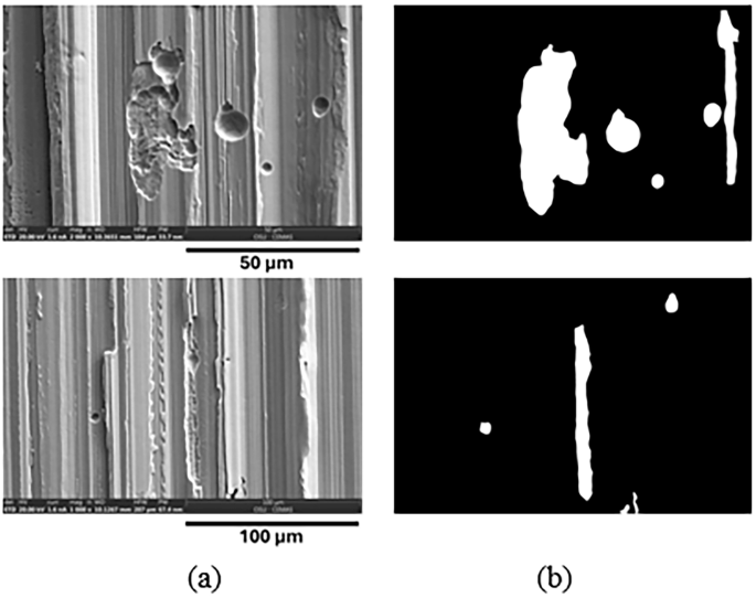
Column (a) shows examples of as collected SEM images. Column (b) displays the corresponding binary masks indicating the corrosion areas.
Implementation
The model was implemented using Pytorch33. The batch size was set to 8 for training. The parameters were updated by Adam optimizer34. The initial learning rate was 1×10⁻³, and the weight decay was 5×10⁻⁴. The analysis was conducted on a single Tesla V100 graphics processing unit. The training process was conducted in two steps. First, the model was trained on the PIS24 dataset for 300 epochs, initialized with pre-trained weights on MS COCO26. In the second step, the model was further trained on the newly constructed CSM dataset for an additional 300 epochs. In the inference stage, we used the testing data from the CSM database and obtained the corrosion segmentation results from the model. Additionally, the quantitative evaluation metrics were also calculated by comparing the predicted results with the ground truth.
To enhance the diversity of the training data and improve the predicting capability of the model, the data was augmented by rotating at 0o, 90o, 180o, 270o and flipping. The augmentation was implemented by a combination of rotations with horizontal, vertical, and dual axis flips at each angle. Additionally, random cropping, brightness adjustment, and resizing were adopted. Specifically, the augmentation process included: a 50% probability of horizontal flipping, random cropping within a range from 0 to 20%, random rotations from -15 to 15 degrees, random sharing from -5 to 5 degrees both horizontally and vertically, random brightness adjustment within a range from -25% to 25%, and random exposure adjustment within a range from -25% to 25%.
As shown in Fig. 8, the training and validation loss curves help assess the generalization performance of the model given the limited dataset of 84 labeled instances. While the dataset is relatively small, the model benefits from pretraining on a large external dataset, and the loss curves show no signs of overfitting. The training loss converges around epoch 300, and the validation loss approaches zero without divergence, indicating consistent learning rather than memorization. Furthermore, on the training set of 75 images, the precision, recall, and mAP metrics show stable and consistent performance, again supporting the robustness of the implementation under data-limited conditions.

The first row shows the training loss curves with training halted after 300 epochs. The “box_loss” and “cls_loss” refer box IoU loss and box classification loss. The “seg_loss” indicates instance segmentation loss. The “obj_loss” is the averaged total loss. The y axis is the value of loss. The second row illustrates the precision, recall and mAP performance curves on the training set. The y axis is the metric value of performance.