
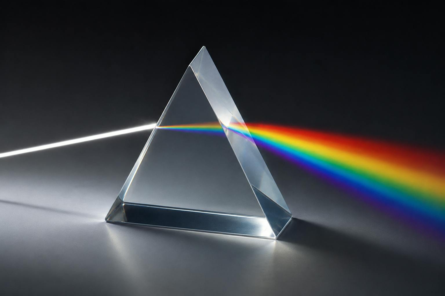
To understand algorithms that control our digital life, we must first understand how they percieve what we call reality.
Everything I write, it is written to draw either a parallel to machine learning, or directly about it. In this series – not really sure how many pieces will fall under it – we will tackle various beliefs and assumptions, short and sweet, with the hope that we either strengthen our understanding or simply revisit what we already know. The series is basically going to be: what is X?This is the first piece in that, and I hope it does not turn out to be complete shite.
Rant
There is a bit of irony in writing this piece though – I am colorblind. To be specific, I am Deutan. This means I struggle with green-red. In the complete absence of green cones green looks beige and red and orange Brown. Yellow and green appear more red if there is a deficiency. Purple and blue also look similar.
But no one better than me to write/rant about colours as well, no?
I have often wondered why we have the insane naming convention for colours. Quite often, I fallback to say well why say teal when you can say its blue and green, cuz I can see it is blue and green, why must I remember it is teal? Why should I remember these useless names.
Its a color, and its giving blue, and its also giving green, so its from blue-green family, yes I can see why it is not completely blue and yes it is not completely green, but it is still from the blue family, and it is still from the green family. And it is closer to being blue than it is to being green (but thats just me)
my comment on the colour ‘Teal’
We humans love breaking things down and giving them names, because it enables higher functionality for us. We have broken colors down to Red, Green, Blue as primary, and then we’ve got secondary colours, and this wasn’t enough so we said hey you know what we want another name and we have Tertiary colours too.
To the model that is being trained to name the colours, how is it viewed – better still to ask: how does it discriminate between different colours?
But before we start off in that direction, lets first make fun of colours.
Understanding Colours
First off, what are colours? Colours are simply our eyes percieving the different wavelengths of light, simulating the cone cells in our eyes. Do you realize what this means? It means two people that can percieve the full spectrum can still see the same color differently. We taste the same food differently, we hear the same music differently, and indeed, we see the same colour differently. This is not obvious until you notice how people percieve the world around them, so go out, touch grass, and make friends, and you will truly appreciate the uniquness of each human being.
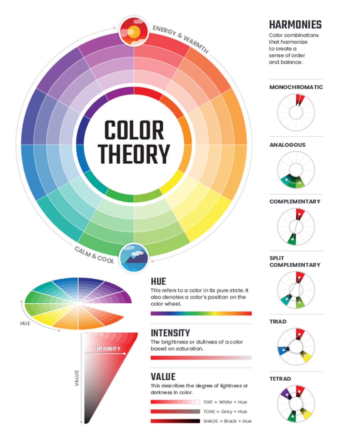 An excellent article from Pavilion
I realized this once, then twice, and then again. I come to realize this every now and then, because otherwise it converts into a fact I know and neurons around it don’t really get activated until some conversation has friction around perception – like I would say do you not notice how clean the roads are here versus back home (even if you take the Middle East which is quite clean in comparison to back home, it still has too much dust – I doubt they can do much about that given its a desert). But, to some, dust does not bother them and they do not see it as unclean. But if you have played too many games like I have, your idea of graphics is associated with the kind of roads you would see in Forza or GTA, and so obviously the roads of the west would appeal more to my sensors.
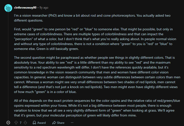 This right here is perhaps the best comment on this topic
Are we in too deep?
And then there is the fact that when we talk about colours, we talk about associations too. The colour red for example, to some its romantic, to some its warfare, to some its the colour of passion. The association might in itself change the way you imagine the colour and affect your perception of it when you are exposed to it – on the lips of a loved one it is romantic, on the airbag after an accident it is a tragedy, on the sky it is an apocalypse, and so on.
We are red inside, but the world we percieve is mostly blue – the sky, the oceans. The sun is yellow, the stars are sparkling white, and in between all of that, we exist, we observe, and we showcase our art in the form of unique architectures and even more unique colour ranges – on our buses, our trains, our cars and our roads that are asphalt grey. The forest is green, and I am told we – the human race – can see more shades of green than any other colour.
You can find this video here, its from a scene from Season 1, Fargo, where Lorne asks the police officer a rhetorical question; did you know that the human eye can see more shades of green than any colour, and poses to him a question at the end; why?
To be fair, the conclusion for ‘why’ in the minds of the masses is that it is due to the fact we were apex predators who spent a great deal of time in the jungles. “Our primate ancestors evolved this trait to survive in dense, natural environments. Being able to distinguish between countless shades of foliage meant they could easily spot hidden predators, find tender, edible plants, and pluck out ripe fruits against the green backdrop.” – an excrept from nhpr
Without further ado, lets build a small neural network (CNN), introduce non linearity (ReLU), and then decode what the filters it built are being used for.
A tidbit before we begin – just because I am feeling the need to mention it -The Universal Approximation Theorem states that a feed-forward neural network with even a single hidden layer can approximate any continuous function to arbitrary precision. Also, there was a longheld belief that NN’s could not even do XOR. Now look at us. Time flies, does it not? hehe.
Dissecting Colours with ML?
I have taken this colour dataset from kaggle to get started.
First, we import some libraries, and then randomly view images.
Manually viewing a few images have made me realize not all the images are of the same dimensions, so lets fix that next.
# Define the base directory where the images are located
base_dir = './training_dataset'

# Get a list of all color categories (subdirectories) in the base directory
color_categories = [d for d in os.listdir(base_dir) if os.path.isdir(os.path.join(base_dir, d))]

if not color_categories:
    print(f"No color categories found in '{base_dir}'. Please ensure the path is correct and the dataset is unzipped.")
else:
    print(f"Found {len(color_categories)} color categories: {', '.join(color_categories)}\n")

    for category in sorted(color_categories):
        category_path = os.path.join(base_dir, category)
        images_in_category = [f for f in os.listdir(category_path) if f.lower().endswith(('.png', '.jpg', '.jpeg', '.gif', '.bmp'))]

        if images_in_category:
            random_image_name = random.choice(images_in_category)
            random_image_path = os.path.join(category_path, random_image_name)
            print(f"Displaying a random image from category: {category}")
            display(Image(filename=random_image_path, width=200)) # Display image with a fixed width for better visualization
            print("\n") # Add a newline for better spacing between categories
        else:
            print(f"No images found in category: {category}\n")
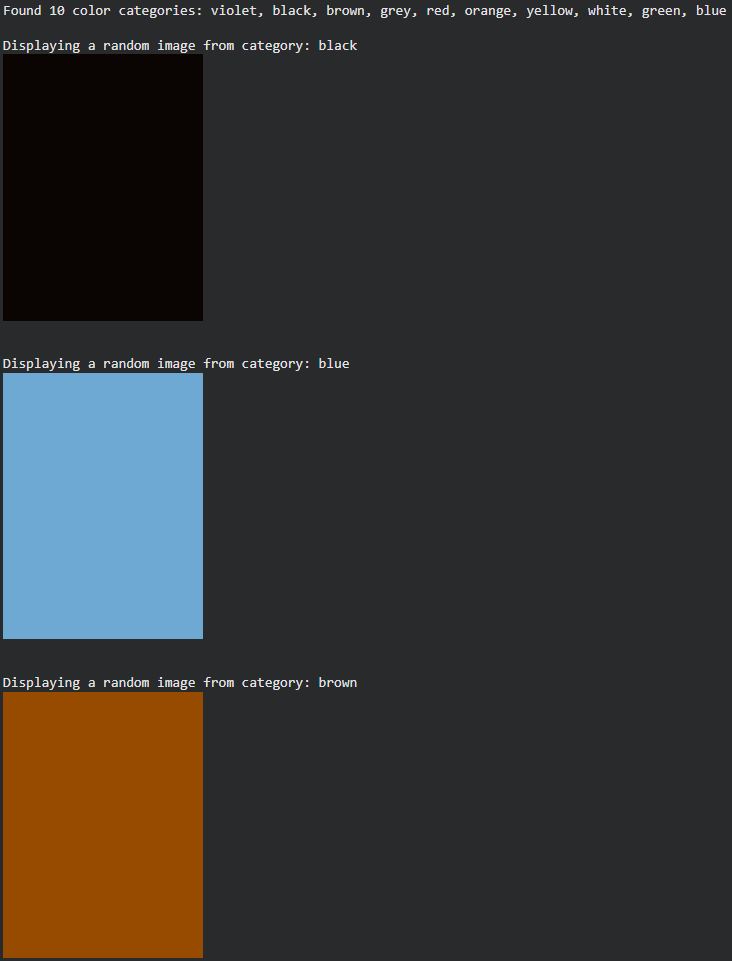
With the code below, we iterate over all of our images, and resize them to 128 x 128 in a new directory.
from PIL import Image
import os

input_base_dir = './training_dataset'
output_base_dir = './resized_training_dataset'
target_size = (128, 128)

os.makedirs(output_base_dir, exist_ok=True)

print(f"Resizing images from '{input_base_dir}' to '{output_base_dir}' with dimensions {target_size}...")

for root, dirs, files in os.walk(input_base_dir):
    for file in files:
        if file.lower().endswith(('.png', '.jpg', '.jpeg', '.gif', '.bmp')):
            input_path = os.path.join(root, file)

            # Create corresponding output directory structure
            relative_path = os.path.relpath(root, input_base_dir)
            output_dir = os.path.join(output_base_dir, relative_path)
            os.makedirs(output_dir, exist_ok=True)

            output_path = os.path.join(output_dir, file)

            try:
                with Image.open(input_path) as img:
                    img_resized = img.resize(target_size, Image.LANCZOS)
                    img_resized.save(output_path)
            except Exception as e:
                print(f"Error processing image {input_path}: {e}")

print("Image resizing complete.")
We can take a peek at what our image spectrum per colour looks like by putting it on a grid (this is not the entire range though).
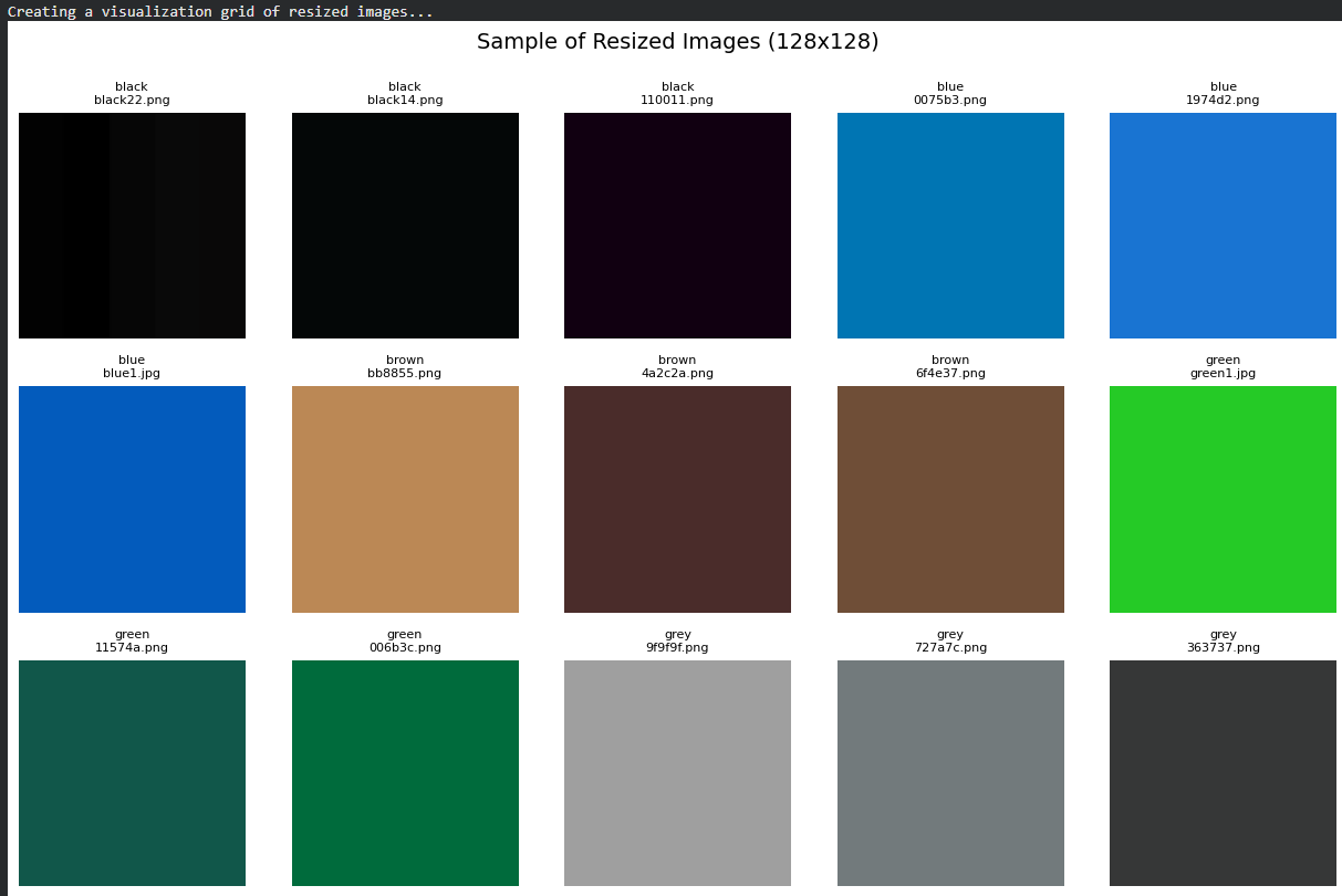
Great. Lets make it ready for model training, split it into train-val as well while we are at it.
import tensorflow as tf

# Define image dimensions and batch size
img_height = 128 # Matching the target_size used for resizing
img_width = 128
batch_size = 8

# Define the directory containing the resized images
data_dir = './resized_training_dataset'

print(f"Loading training data from: {data_dir}")

# Load the training dataset (80% of data)
train_ds = tf.keras.utils.image_dataset_from_directory(
    data_dir,
    validation_split=0.2,
    subset="training",
    seed=123,
    image_size=(img_height, img_width),
    batch_size=batch_size
)

print(f"\nLoading validation data from: {data_dir}")

# Load the validation dataset (20% of data)
val_ds = tf.keras.utils.image_dataset_from_directory(
    data_dir,
    validation_split=0.2,
    subset="validation",
    seed=123,
    image_size=(img_height, img_width),
    batch_size=batch_size
)

# Get class names
class_names = train_ds.class_names
print(f"\nFound {len(class_names)} classes: {class_names}")

# Configure dataset for performance
AUTOTUNE = tf.data.AUTOTUNE

train_ds = train_ds.cache().prefetch(buffer_size=AUTOTUNE)
val_ds = val_ds.cache().prefetch(buffer_size=AUTOTUNE)

print("\nDatasets prepared successfully. Ready for model building and training.")
Here, we have split it up into train and validation, where validation is 20% of our data. You can imagine if there were 10 images in each category, 2 of them now sit inside validation. The challenge with just having train-val and not test as well is that while the model trains, it gets some level of understanding of what is in the validation when it scores poorly so in a way, the validation dataset dictates the final models outlook without having exposed its content (For example, you adjusting the model configuration based on its performance on the validation set). With a test set, it does not become part of this cycle and therefore we should have at least 10% of our dataset sit there as well.
Ignore the autotune, its just a functionality of Tensorflow to manage the number of parallel calls when processing input data and avoiding bottlenecks at training time while serving this pipeline.
With Keras, you can build a model in many ways, the most common are Sequential and Functional. There is also model subclassing. Based on complexity, you go higher up this spectrum. For us, sequential should do just fine. You can read more in detail here.
With a very simple model (in the olden days, this might have gotten us lynched for calling it simple given the sophistication hidden behind the framework)
num_classes = len(class_names)

model = Sequential([
    Input(shape=(img_height, img_width, 3)), # Explicitly define Input layer
    layers.Rescaling(1./255),
    layers.Conv2D(4, 5, padding='same', activation='relu'),
    layers.MaxPooling2D(),
    layers.Conv2D(8, 5, padding='same', activation='relu'),
    layers.MaxPooling2D(),
    layers.Conv2D(16, 5, padding='same', activation='relu'),
    layers.MaxPooling2D(),
    layers.Flatten(),
    layers.Dense(16, activation='relu'),
    layers.Dense(num_classes, activation='softmax')
])

model.summary()
Its only 3 layers deep, with a fully connected layer at the end before the classification layer (which in this case would have 10 options). Our first layer has about 4 units, and we use multiples of 4 for the subsequent layers. Finally, our FC layer has about 16 neurons to re-represent the knowledge from the convolutional overlords.
Recap: Core DL
Softmax limits the output vector to a sum of 1. This means, given the representation from the prior layer, how can we map it to the classes such that the most relevant layer has the highest value while all the others are minimal.
Maxpooling simply takes the most informative part from the filter and brings it forward.
The reason for why we increase the units progressively (4, 8, 16) can be a design choice and other styles can be tried out as well (equal sized, inverted, triangle etc) but in this case, my assumption that guided this was the fact that our earlier layer has a less complex task, it has access to the actual image, and usually the earlier layers only pick apart edges and corners etc but later layers have a much more complex task of dissecting what other factors define the supplied representation.
model.compile(
    optimizer='adam',
    loss=tf.keras.losses.SparseCategoricalCrossentropy(from_logits=False),
    metrics=['accuracy']
)
Nothing unique to see here, picked the most popular optimizer ‘adam’ which is basically how we traverse the error graph and minimise loss. The loss here is SparseCategoricalCrossEntropy which is just saying I am lazy and do not want to one hot encode my output space. With this loss, we can supply integer labels (e.g., black = 0, blue = 1, brown = 2, etc.).
epochs = 10
history = model.fit(
    train_ds,
    validation_data=val_ds,
    epochs=epochs
)
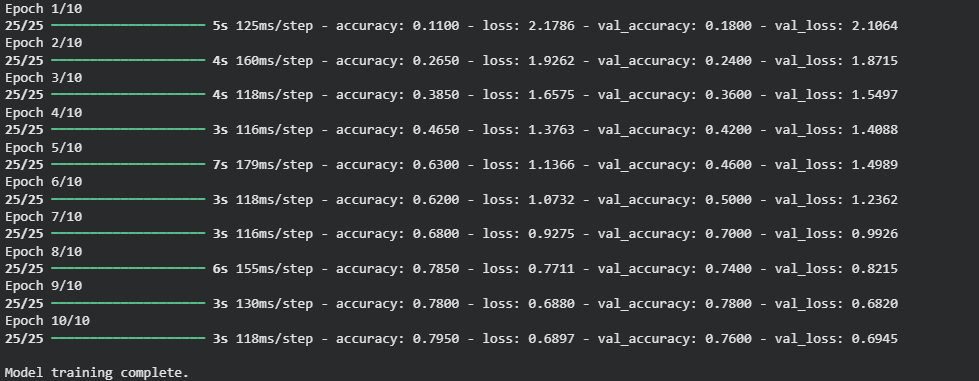
We only go 10 epochs deep (although we can end earlier with EarlyStopping, or be even more clever with adaptive LR and other techniques – but that really is not the focus here so I have avoided doing that).
An epoch is simply the journey of fully traversing the dataset. In this case the 80% of the total dataset that was present in the training dataset seen once would mean 1 epoch, and the batch size we picked earlier decides how many times would we update our weights/beliefs/priors during a single epoch. For example, if we had a 100 images in the training dataset, and a batch size of 8, we would update 100/8 times in one epoch, and in total we have 10 epochs therefore the total times we update our models belief system is 10 * 100/8 or 125 times.
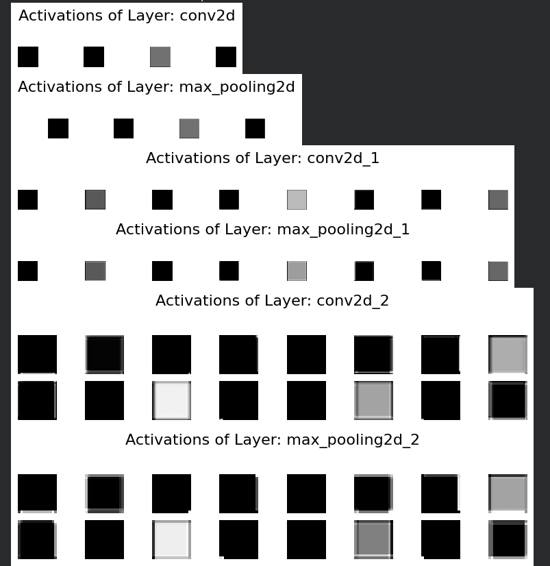
Now, lets visualize what our layers have learned to see how the model sees colours.
On yellow:
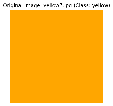
Our model outputs this:
 Feature Map
The clever part about layers is that because they are not harcoded (like you would a filter – gaussian/Sobel/Laplacian), they are free to find features as they please. You would often read about early layers being edge detectors – but what about when an image has no edge and is – like in this case – a solid colour? Well, it then tries seemingly to create filters around different colour channels and their combinations / intensity / hue etc – for example how a muted yellow and a bright yellow are one and the same but differ from light green or light brown etc.
The Feature Map shown here is simply: each square is a ‘highlight map’ showing where and how intensely a particular filter responded to the input image of ‘Yellow’.
Black Areas mean low activation (meaning they might light up for a different colour or perhaps a different shade of Yellow) – but essentially going ‘our opinion is that we do not have an opinion on this’ – and that in itself is an opinion telling us something about the image.
White Areas mean high activation. This basically means these filters have strong opinions and feelings and are activated when this colour is shown.
Intermediate Shades of Grey are basically moderate activations, and have opinions about the image but not really strong with their feelings about it.
Also, if you notice the later layers have a bit of a blur around their edges? thats because of convolutions – summaries of the overall pattern and not so easy to decode as say the earlier layers where you might be able to spot an edge detector in action.
Out of curiosity, lets pass the colour ‘Red’ to see how this changes.

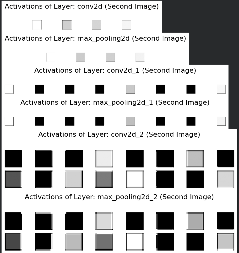
You can immediately notice how different this is by seeing severe activations on the first layer’s filter 1 and filter 4 (column 1 and column 4), and then it propogating downards to showcase a completely different activation map.
Okay. We can see how differently they feel about different colours. But the more important thing is to understand how much they differ from us – Then again, if we were to examine how our brains synapses respond at different colours across different people it would obviously be complex and hardcore as well.
I have now actually completely forgotten what the point was of this whole exercise. Maybe I wanted to say, do not be attached or fooled or impressed by the ability of infinite monkeys typing shakespeare.
You can check the notebook here.
You can get the dataset from Kaggle.
Thats it, see you next time!


