

Dataset description
The present study, conducted a retrospective analysis on a hospital-based registry database for COVID-19, from February 25, 2020, to November 15, 2021. The dataset consisted of patient data obtained from Children Hospital Medical Center, a specialized pediatric referral institution in Tehran, Iran. The sampling protocol received approval from the Ethics Committee of Tehran University of Medical Sciences, Tehran, Iran (IR.TUMS.CHMC.REC1399.069). All methods were performed in accordance with the relevant guidelines and regulations, including the Declaration of Helsinki. Informed consent was obtained from all participants and/or their legal guardians prior to data collection.
The registry database included 93 primary features (Supplementary Table 1) categorized into 4 main classes: demographics (3 features), clinical characteristics (40 features), comorbidity history (6 features), laboratory results (43 features) and an outcome variable indicating severity status (0: Non-severe, 1: Severe). Quantitative parameters were measured numerically, while nominal parameters were recorded as binary responses (1: Yes or 0: No). Supplementary Table 2 describes dataset structure and class distribution.
Severe COVID-19 was defined based on objective clinical outcomes adapted from the World Health Organization (WHO) COVID-19 clinical progression scale34with severe disease classified by the occurrence of one or more of the following critical endpoints: ICU admission for close monitoring or advanced support, intubation for respiratory failure, mechanical ventilation for respiratory support, and death attributable to COVID-19 complications. These criteria were chosen to reflect clinically significant disease progression and align with prior peer-reviewed studies35,36,37. This severity classification was used as the outcome variable (Y) in the supervised learning models, where the goal was to distinguish between severe and non-severe cases based on the predictor variables (Supplementary Table 3).
Each patient was registered only once in the dataset, with only the first set of laboratory results collected during their initial admission being considered. Demographic and comorbidity history information was sourced from medical records or directly from patients and their companions. Clinical features were documented upon admission, and laboratory tests were conducted during the initial hours of hospitalization. Patients were initially assessed in the hospital’s emergency department before being admitted and subsequently transferred to the appropriate hospital wards. Laboratory tests were conducted during the first hours of their hospital stay, and the results were integrated into their medical records. Finally, Laboratory results were integrated into the patients’ medical records.
Chest CT imaging was conducted only when requested by a specialist. The identified CT features of COVID-19 included ground-glass opacities, consolidations, opacity distribution, pleural effusion, fibrosis, and nodules. Additionally, the extent of bilateral lung involvement and the number of affected lobes were evaluated. All CT images were independently reviewed by two radiologists to ensure accuracy. Any discrepancies between the initial reviews were resolved through consultation with a senior radiologist.
Data pre‑processing
In the present study, data pre-processing was undertaken prior to training the machine learning algorithms in order to addressing irrelevant and unreliable data. Initially, records with more than 60% missing data were excluded from the dataset. For the remaining records, missing values in binary variables were imputed using logistic regression, while missing values in continuous variables were imputed using predictive mean matching using ‘mice’ package38 in R environment. All continuous variables were standardized using Z-score normalization to ensure consistency across features. This transformation was performed using the ‘step_normalize’ function from the ‘recipes’ package and was applied after multiple imputation to maintain data integrity.
As previously indicated, the present study uses chest CT scores to show each patient’s level of pulmonary involvement. Initially, two-digit codes were used to reflect different CT findings, such as ground-glass opacities, consolidation, bilateral lung disease, more than two lobes affected, pulmonary nodule, pleural effusion, lymphadenopathy, empyema, and fibrosis. Each variable was coded as 0 (No) or 1 (Yes). To generate a composite score that exhibited the overall degree of pulmonary involvement, the binary chest CT score values were combined into a single score ranging from 0 to 9 by summing the individual binary values for each patient.
Also, to properly include categorical variables such as blood group in the machine learning models, the blood group variable was transformed into dummy variables. This approach allows the model to handle categorical data more effectively by converting each category into a binary variable. The ‘fastDummies’ package39 was used to perform this transformation. This transformation ensured that the categorical information was appropriately represented in the model, improving its ability to capture the relationship between blood group and COVID-19 severity.
Only positive RT-PCR COVID-19 cases were included in the study. Exclusion criteria encompassed negative RT-PCR COVID-19 test results, unknown dispositions, over 60% missing data, and patients older than 18 years old. Inclusion and exclusion criteria for the study are schematically shown in Fig. 1.
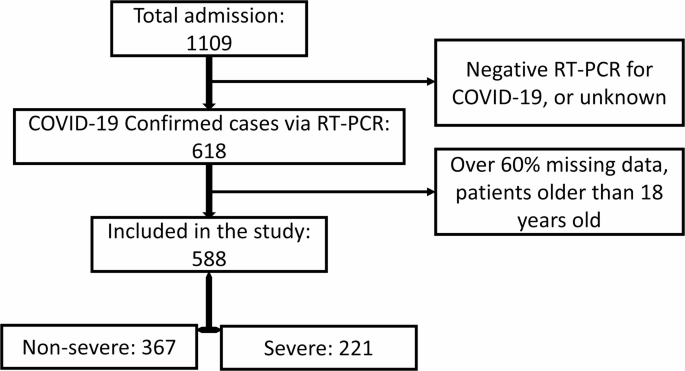
Patient selection flowchart. The flowchart details the selection process for the patient included in the study. From 1,109 initial admissions, 588 pediatric patients with confirmed COVID-19 via RT-PCR were included after applying exclusion criteria. The final patient group was divided into 367 non-severe and 221 severe cases, which were used for subsequent predictive modeling analyses.
Feature selection
To reduce the risk of overfitting in ML algorithms, selecting the key variables that have a strong correlation with the outcome variable is essential. This research, identified important variables for predicting COVID-19 severity through Generalized Boosted Models (GBM) and Random Forest (RF) models using the ‘SLScreenExtra’ package40. To further refine the feature set, highly correlated variables were excluded with a correlation coefficient greater than 0.75 using the ‘findCorrelation’ method from the ‘caret’ package41. The variables selected through this process are listed in Table 2, which can be found in the Results section. This careful selection process was designed to enhance the predictive accuracy and robustness of the models by focusing on the most relevant predictors.
Model training and evaluation
Present research utilized several types of ML algorithms, including Neural Network (NN), Generalized Boosted Models (GBM), Random Forest (RF), Recursive Partitioning and Regression Trees (RPART), k-Nearest Neighbors (k-NN), and kernel support vector machines (KSVM), to forecast the severity of COVID-19 in children. A variety methodological approaches and their proved effectiveness in medical predictive modeling were the basis for the selection of ML algorithms for this study. Neural Networks were included due to their ability to model complex, non-linear relationships42,43. GBM and RF were selected for their robustness in handling high-dimensional data and their ensemble nature, which improves prediction accuracy44,45. RPART was chosen for its interpretability, allowing for clear decision-making processes46. k-NN was included due to its simplicity and effectiveness in classification tasks47. KSVM was selected for its powerful classification capabilities, particularly in high-dimensional spaces. It is particularly useful for binary classification tasks, such as predicting severe vs. non-severe cases48. By employing a diverse set of algorithms, the study aimed to leverage the unique strengths of each method, ensuring a comprehensive and robust prediction model for COVID-19 severity in children. Since the outcome variable was binary (severe vs. non-severe), all models were trained as binary classification models, optimizing performance based on metrics such as AUC.
Each model was trained using the “SuperLearner” package49 with specific libraries corresponding to each algorithm (e.g., SL.nnet for NN, SL.gbm for GBM), utilizing 70% of the dataset as a randomly allocated training set. The models were then evaluated on a 30% holdout set, with predictions converted to binary outcomes based on a threshold of 0.5. A 70:30 train-test split was used to evaluate all machine learning models in this study. This ratio was chosen to ensure that a sufficient amount of data was available for training while preserving a robust holdout set for performance evaluation. Given the dataset size and the relative class imbalance, alternative splits such as 80:20 or 90:10 were avoided to prevent reduced evaluation reliability and potential overfitting. Furthermore, the SuperLearner ensemble employs internal 10-fold cross-validation, which inherently supports robust performance estimation and generalization. Confusion matrices were used to assess the performance of each model, providing metrics such as accuracy, sensitivity, and specificity. Hyperparameter tuning was not performed for individual machine learning models, and default parameters were used for both the base learners and the SuperLearner ensemble. The SuperLearner framework dynamically optimizes model weights, reducing the need for manual tuning while ensuring that the ensemble effectively leverages the predictive strengths of its components. Given the dataset size, this approach helps prevent unnecessary complexity and potential overfitting. The default parameters used for each individual algorithm and the SuperLearner ensemble in this study are detailed in Supplementary Table 4. Also, to address the moderate class imbalance (62% non-severe vs. 38% severe), we considered potential effects on classifier sensitivity and specificity. However, no resampling strategies (e.g., oversampling, SMOTE, undersampling) or class weighting adjustments were applied during model training. This decision was informed by two factors: (1) the imbalance was not extreme, and (2) performance metrics such as sensitivity, specificity, and AUC remained well-balanced across models. Importantly, ensemble modeling via SuperLearner with internal cross-validation was used to further mitigate the impact of class imbalance and enhance generalizability. Nonetheless, future studies may benefit from applying and comparing resampling or cost-sensitive learning techniques to explore their potential performance gains, particularly in more imbalanced settings.
Mathematical overview and terminologies of machine learning models
To improve transparency, this subsection provides the fundamental formulations and terminologies for the machine learning models used in this study:
Random Forest (RF).
RF is an ensemble of decision trees trained on bootstrapped subsets of the data. The prediction for classification is given by:
ŷ = mode(T₁(x), T₂(x), …, Tₙ(x)).
where Ti(x) is the prediction from the i-th decision tree.
Gradient Boosted Machines (GBM).
GBM builds trees sequentially, where each new tree minimizes the residual error of the previous ensemble. The model prediction is given by:
where hₘ(xi) is the prediction from the m-th tree, and γₘ is the step-size (often scaled by the learning rate).
Support Vector Machines (SVM).
SVM seeks to find a hyperplane that maximizes the margin between classes. The decision function is:
where αi are support vector coefficients, yi are class labels, K(xi, x) is a kernel function (e.g., RBF), and b is the bias term.
Neural Network (NN).
A feedforward neural network computes predictions as:
ŷ = f(W₂·σ(W₁·x + b₁) + b₂).
where W₁, W₂ are weight matrices, b₁, b₂ are biases, σ is an activation function (e.g., ReLU, sigmoid), and f is the final output function (e.g., softmax).
SuperLearner (SL) Ensemble.
The SuperLearner model combines multiple base learners through weighted averaging:
ŷ_SL=Σj=1Jαjŷj(x)
where ŷj(x) is the prediction from the j-th base learner, and αj is the optimized weight assigned to each learner.
Unlike fixed ensemble strategies such as bagging (e.g., Random Forest) or boosting (e.g., GBM), the SuperLearner framework implements a stacking-based approach, using cross-validation to learn the optimal weighted combination of diverse base learners. This method allows the ensemble to adaptively exploit the strengths of each algorithm, improving overall predictive performance and generalizability.
Each model’s mathematical foundation enhances interpretability, particularly when combined with feature importance or XAI analysis. These models were implemented using default parameters (see Supplementary Table 4), and trained on a 70/30 split of the dataset.
Cross-Validated superlearner (CV.SuperLearner)
The CV.SuperLearner algorithm was employed to enhance predictive performance by leveraging the strengths of individual models. This ensemble method combined multiple algorithms, including NN, RF, GBM, RPART, k-NN, and KSVM. The ensemble model was trained using a 10-fold cross-validation approach to estimate the risk and compare the performance of the different algorithms. Risk estimates from the CV.SuperLearner model were summarized and visualized, offering insights into the distribution of the best single learner across external cross-validation folds. Supplementary Table 5 shows summary of machine learning models used in this study and included in the ensemble model.
Data analysis and model training were conducted using R version 4.4.150ensuring robust and reproducible results through a well-established statistical computing environment.


