Achieving interpretable machine learning by functional decomposition of black-box models into explainable predictor effects

Machine learning (ML) has increased greatly in both popularity and significance, driven by an increase in methods, computing power and data availability¹, making it an useful tool in the development of artificial intelligence (AI). On May 29, 2025, a search on Web of Science for publications including the term “machine learning” yielded more than 474,000 results, corresponding to an average annual increase by more than 22% since 2006. ML models are often characterized by their high generalizability, making them particularly successful when used for supervised learning tasks like classification and risk prediction. In recent years, ML models based on deep artificial neural networks (ANNs) have led to groundbreaking results in the development of high-performing prediction models².

The high prediction accuracy of modern ML models is usually achieved by optimizing complex “black-box” architectures with thousands of parameters. As a consequence, they often result in predictions that are difficult, if not impossible, to interpret. This interpretability problem can hinder the use of ML in fields like medicine, ecology, and insurance, where an understanding of the model and its inner workings is paramount to ensure user acceptance and fairness³. In a recent environmental study, for example, we explored the use of ML to derive predictions of stream biological condition in the Chesapeake Bay watershed (CBW) of the mid-Atlantic coast of North America⁴. Clearly, if these predictions are intended to inform future management policies (projecting, e.g., changes in land use, climate, and watershed characteristics), they need to be interpretable in terms of relevant features as well as the directions and strengths of the feature effects. We will return to this example below in order to illustrate our proposed methodology.

Interpretable machine learning

In recent years, the need for understanding ML models has boosted research in the field of interpretable machine learning (IML^3,5,6). In this field, interpretability is commonly defined as “the degree to which a human can understand the cause of a decision”⁷. A related concept considered separately in some works is explainability, which describes “the internal logic and mechanics that are inside a ML system”⁸. Because the methodology presented in this work applies to both concepts, we will not distinguish between the two.

The focus of this paper is on IML for supervised learning tasks, which involve a set of features X = {X₁, …, X_d} to derive predictions of a qualitative or quantitative outcome variable Y. Denoting the model (i.e., the prediction function) by \(F(X)\in {\mathbb{R}}\), interpretability can generally be achieved in two ways: The first approach is to impose an interpretable structure on F during the learning process (“model-based” or “by-design” interpretability^5,6). An example of this approach is the least absolute shrinkage and selection operator⁹, which, in its basic form, assumes F to be linear in the features. Consequently, each feature effect is interpretable in terms of a real-valued coefficient. The second approach, which is particularly applicable to black-box models, aims to achieve interpretability by post-processing an already learned prediction model (“post hoc” interpretability^6,10). Here we will consider model-agnostic post-processing methods, which can be applied to a broad range of prediction functions regardless of the ML method applied to the training data³. Popular examples of model-agnostic methods include partial dependence plots (PDP) and accumulated local effects (ALE) plots. The underlying principle of these methods is to measure the variability of the prediction function F with respect to changes in subsets of the features X (an approach that is closely linked to the concept of sensitivity analysis in numerical and nonlinear regression modeling^11,12).

While PDP and ALE plots have become established methods in IML, they are not without limitations. For example, PDP have been criticized for ignoring the correlations between the feature of interest and the other features, relying on data points with a very low probability of being observed. This “extrapolation” issue may result in misleading effect estimates when the features are correlated³. Similarly, PDP may hide possible interaction effects of the features, a problem that can be alleviated by individual conditional expectation plots in some cases^3,13. While ALE plots avoid extrapolation of the data¹⁴, Grömping¹⁵ observed that these plots do not generally identify the linear shapes of the main effects in a linear prediction model. As a consequence, the feature effects depicted by ALE plots may show systematic deviations from the respective effects in the model formula (for which an explanation is sought). The method proposed in this paper is not affected by these issues: It avoids hiding feature interactions by explicitly including these terms in the estimation procedure and is solely based on the multivariate feature distribution to avoid extrapolation. Furthermore, it does not alter the shapes of the main effects in a linear model.

Functional decomposition

The basic idea of our method is to achieve interpretability by decomposing the prediction function F (depending on all features X) into a set of simpler (“better interpretable”) functions depending on subsets of the features only. More specifically, let ϒ = {1, …, d} the set of feature indices and \({\mathcal{P}}(\Upsilon )\) the power set (i.e., the set of all subsets) of ϒ. Then F can be decomposed into a sum of functions

where \(\mu \in {\mathbb{R}}\) is an intercept term and, for any \(\theta \in {\mathcal{P}}(\Upsilon )\backslash {{\emptyset}},{X}_{\theta }\) denotes the subset of features with indices θ. For example, if d = 3 and θ = {1, 3}, then X_θ is given by {X₁, X₃}. Accordingly, the intercept term can be defined as \(\mu ={f}_{{{\emptyset}}}\). Note that the last sum in Eq. (1) consists of only one summand.

In IML, the main focus is usually on the subset of functions f_θ with ∣θ∣ = 1 (“main effects”, first sum in Eq. (1)) and ∣θ∣ = 2 (“two-way interactions”, second sum in Eq. (1)). For main effects, f_θ depends on only one feature X_j, j ∈ ϒ, allowing for a simple graphical analysis that plots the values of f_θ(X_j) against the values of X_j. For example, in the aforementioned study on stream biological condition, the main effect of 30-year mean annual precipitation shows a positive association between the amount of precipitation and the predicted values of stream condition (see Fig. 3 below). Two-way interactions, on the other hand, can be visualized using heatmaps or contour plots. For example, Fig. 4 below presents a plot of the interaction between the elevation of the sample sites and the percentage of upstream catchment area as developed, showing elevations at which land use for development leads to low biotic integrity. As demonstrated by these examples, both main effects and two-way interactions allow for simple graphical interpretations of the respective feature effects, whereas the functions f_θ with ∣θ∣ > 2 (termed “multivariate feature interactions”) constitute the less interpretable parts of F.

This paper presents a novel approach to specify and compute the functions f_θ, given a fixed (possibly black-box) prediction function F. The proposed method also allows the measurement of the “degree of interpretability” by quantifying the importance of the main and two-way interaction effects in Eq. (1). We emphasize that our methodology is designed to decompose the prediction function F but not to learn it from a set of data. Accordingly, we assume that F is not subject to sampling variability but has been derived previously by the application of some ML method. Our method is based on regularity conditions that are similar to those described by Hooker¹⁶; however, we consider a different type of functional decomposition and also employ a different computational methodology.

Conditions on the features and the prediction function

It is clear from Eq. (1) that the functions f_θ are not uniquely defined. For example, let d = 2, μ = 0, and F(X₁, X₂) = X₁ + X₁ ⋅ X₂. Then the sets of functions {f₁(X₁) = X₁, f₂(X₂) = 0, f₁₂(X₁, X₂) = X₁ ⋅ X₂} and {f₁(X₁) = 0.5 ⋅ X₁, f₂(X₂) = 0, f₁₂(X₁, X₂) = 0.5 ⋅ X₁ + X₁ ⋅ X₂} both satisfy Eq. (1). As a consequence, further assumptions are needed to derive a unique representation of Eq. (1).

Our first set of assumptions is on the features X = {X₁, …, X_d}. In line with Hooker¹⁶, we consider the features as real-valued random variables, assuming that X₁, …, X_d are defined on a joint probability space with probability function P_X. We further assume that each X_j, j ∈ ϒ, has bounded support. Note that these are rather weak assumptions in practice, allowing X to include both continuous and categorical features (the latter encoded by sets of dummy variables).

Regarding the functions in Eq. (1), we assume that each f_θ, and also F, is square integrable with respect to P_X. Again, this is a rather weak assumption, as square integrable functions emerge from many popular ML methods. They include, for instance, the piecewise prediction functions obtained from random forests and tree boosting, and also many ANN predictors after transformation by a sigmoid activation function. Following Hooker¹⁶, we define the variance of \({f}_{\theta },\theta \in {\mathcal{P}}(\Upsilon )\backslash {{\emptyset}}\), by \({\sigma }_{\theta }^{2}=\int{f}_{\theta }^{2}({X}_{\theta })d{P}_{X}\), the variance of F by \({\sigma }_{F}^{2}=\int{(F(X)-\mu )}^{2}d{P}_{X}\), and the covariance of f_θ and \({f}_{{\theta }^{{\prime} }},\theta ,{\theta }^{{\prime} }\in {\mathcal{P}}(\Upsilon )\backslash {{\emptyset}}\), by \({\sigma }_{\theta {\theta }^{{\prime} }}=\int{f}_{\theta }({X}_{\theta }){f}_{{\theta }^{{\prime} }}({X}_{{\theta }^{{\prime} }})d{P}_{X}\). Without loss of generality, we assume that each \({f}_{\theta },\theta \in {\mathcal{P}}(\Upsilon )\backslash {{\emptyset}}\), is centered around zero, i.e., ∫ f_θ(X_θ) dP_X = 0¹⁶ (p. 714). Finally, we assume that the functions \({f}_{\theta },\theta \in {\mathcal{P}}(\Upsilon )\backslash {{\emptyset}}\), are linearly independent. This assumption means that each f_θ forms a closed subspace of the Hilbert space of square integrable functions. In practice, it implies that each f_θ carries unique information about F and that all functions f_θ are non-zero.

Generalized functional analysis of variance (ANOVA)

Next, we define a set of requirements to describe the relations between the functions f_θ. Our main requirement is that the summands in Eq. (1) are well separated, meaning that higher-order effects (i.e., functions with large ∣θ∣) do not contain any components of lower-order effects with small ∣θ∣ (see below for a mathematical treatment). In particular, we require that predictive information explained by a main effect is not contained in the higher-order effects that include the corresponding feature (purity criterion, Molnar³, Section 8.4). A related requirement is optimality, meaning that lower-order functions should capture as much functional behavior as possible¹⁶.

To implement the above requirements, Hooker¹⁶ proposed a decomposition termed generalized functional ANOVA. With this approach, the functions in Eq. (1) are required to be hierarchically orthogonal, satisfying the constraints

Hierarchical orthogonality implies that for any given \({\theta }^{{\prime} }\), the effect \({f}_{{\theta }^{{\prime} }}({X}_{{\theta }^{{\prime} }})\) is orthogonal to all higher-order effects f_θ(X_θ) with \({X}_{\theta }\supseteq {X}_{{\theta }^{{\prime} }}\)^16,17. It thus provides an implementation of the purity criterion, ensuring that higher-order effects are uncorrelated with lower-order effects. Furthermore, the constraints in Eq. (2) provide an implementation of optimality because, according to Eq. (2), all lower-order effects \({f}_{{\theta }^{{\prime} }}\) are orthogonal projections of the combined effects \({f}_{{\rm{comb}}({\theta }^{{\prime} },\theta )}:= {f}_{{\theta }^{{\prime} }}+{f}_{\theta }\) onto the respective lower-order subspaces. It follows from the Hilbert projection theorem¹⁸ that the lower-order effects \({f}_{{\theta }^{{\prime} }}\) capture as much of the variance of \({f}_{{\rm{comb}}({\theta }^{{\prime} },\theta )}\) (i.e., as much functional behavior of \({f}_{{\rm{comb}}({\theta }^{{\prime} },\theta )}\)) as possible.

In his original work on generalized functional ANOVA, Hooker¹⁶ specified conditions for the uniqueness of the functions f_θ. He considered a more general definition of the integral in Eq. (2), allowing for weight functions other than the probability density function of X. Based on the same decomposition, Chastaing et al.¹⁹ studied further assumptions on the feature distribution P_X. The authors also introduced a coefficient to measure the importance of individual feature combinations. For each \(\theta \in {\mathcal{P}}(\Upsilon )\backslash {{\emptyset}}\), this coefficient is defined as \({S}_{\theta }=({\sigma }_{\theta }^{2}+{\sum }_{{\theta }^{{\prime} }\ne \theta }{\sigma }_{\theta {\theta }^{{\prime} }})/{\sigma }_{F}^{2}\) (generalized Sobol sensitivity index, Chastaing et al.¹⁹, p. 2427).

Computational challenges

In recent years, functional decomposition has been acknowledged as a key concept in making ML models explainable³. In practice, however, the application of functional decomposition methods remains challenging. This is mainly due to the computational and numerical issues associated with the estimation of the feature effects f_θ. In fact, despite the availability of algorithms to achieve hierarchical orthogonality^16,19,20, state-of-the-art methods still involve systems of equations that are, even for a moderate feature count, “complex and computationally intensive”³. Here we introduce stacked orthogonality, an alternative approach to implement purity and optimality. Based on the conditions of stacked orthogonality, we will present an algorithm to estimate the functions f_θ in a computationally efficient manner.

Functional decomposition with stacked orthogonality

Analogous to generalized functional ANOVA, our method is based on the functional decomposition in Eq. (1). However, instead of the hierarchical orthogonality constraints in Eq. (2), we require the functions f_θ to meet the stacked orthogonality constraints

where k ∈ ϒ denotes the effect level. Throughout the paper, we will use the terms “order” and “level” interchangeably. Unlike hierarchical orthogonality, which requires the effect of each individual feature combination θ to be uncorrelated with higher-order effects, the conditions in Eq. (3) provide a level-wise implementation of the purity criterion: for each level k, the sum of all level-k effects is required to be uncorrelated with the sum of all lower-level effects (including the intercept with \(| {\theta }^{{\prime} }| =0\))—hence the term “stacked orthogonality”. In addition to implementing purity, the constraints in Eq. (3) also provide a level-wise implementation of optimality. This is because, according to Eq. (3), the sum of the “lower-order” effects (with levels <k) is an orthogonal projection of the sum of the “current-order” effects (with levels ≤k) onto the lower-order subspace. It follows from the Hilbert projection theorem that the sum of lower-order effects captures as much of the variance of the sum of the current-order effects (i.e., as much functional behavior at the current level) as possible.

A convenient feature of stacked orthogonality is that the variance of F can be decomposed in a level-wise fashion, giving rise to the calculation of level-wise coefficients of explained variation. More specifically, for each k ∈ ϒ, we define the fraction of \({\sigma }_{F}^{2}\) explained by the k-th level as

By definition, it holds that \(\mathop{\sum }\nolimits_{k = 1}^{d}{I}_{k}=1\) if the stacked orthogonality constraints in (3) are met. Consequently, by calculating I₁ (fraction of \({\sigma }_{F}^{2}\) explained by the main effects) and I₂ (fraction of \({\sigma }_{F}^{2}\) explained by the two-way interaction effects), it is possible to quantify the degree of interpretability of the prediction model F. We emphasize that the definition in Eq. (4) is different from the generalized Sobol sensitivity indices in ref. ¹⁹, as the latter refer to contributions of individual feature combinations \(\theta ,\theta \in {\mathcal{P}}(\Upsilon )\), whereas I_k, k ∈ ϒ, measures the level-wise contributions of all features. For example, in the aforementioned study on stream biological condition, the contribution of the main effects (as measured by I₁) was 80.6%. The contribution of the interaction effects (I₂) was 2.5%, leading to a total of 83.1% model interpretability.

Estimation by neural additive models and post-hoc orthogonalization

As stated above, the application of functional decomposition methods strongly depends on the availability of a user-friendly algorithm to compute the functions f_θ. To arrive at the decomposition in Eq. (1) satisfying the stacked orthogonality constraints, we propose the following three-step procedure:

In the first step, we generate a sample of n data points \({\mathcal{S}}={\{{F}_{i},{X}_{i1},\ldots ,{X}_{id}\}}_{i = 1,\ldots ,n}\), where X_ij, j ∈ ϒ, and F_i = F({X_i1, …, X_id}) denote the j-th feature value and the value of the prediction function, respectively, of the i-th data point. For instance, the data could be sampled from an available set of training data that were used previously for the learning of F. In this case, the probability measure P_X is given by the distribution of the feature values in the training data. Alternatively, one could use a grid of feature values to generate \({\mathcal{S}}\) (corresponding to uniformly distributed features) or some other reference distribution for which an explanation is sought.

In the second step, we use the data generated in Step 1 to obtain initial estimates \({f}_{\theta }^{0}\) of the functions \({f}_{\theta },\theta \in {\mathcal{P}}(\Upsilon )\backslash {{\emptyset}}\). This is done by fitting a neural additive model (NAM²¹) of the form

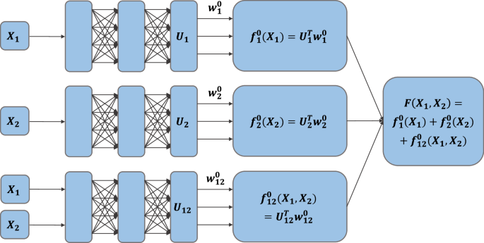
where X_iθ are the values of X_θ corresponding to the i-th data point. Model fitting is performed using a backpropagation procedure, with each function \({f}_{\theta }^{0}\) represented by an ANN depending on the respective feature subset X_θ (see Fig. 1 for an illustration). As demonstrated by Agarwal et al.²¹, NAMs allow for modeling a wide range of functional shapes, exploiting the property of ANNs to approximate general classes of functions arbitrarily well^{22,23,24,25,26,27,28,29,30}. Compared to Agarwal et al.²¹, our only additional requirement (needed for Step 3 below) is that all ANNs in Eq. (5) are linear in their output layers. More specifically, we require each vector \({{\bf{f}}}_{\theta }^{0}={({f}_{\theta }^{0}({X}_{1\theta }),\ldots ,{f}_{\theta }^{0}({X}_{n\theta }))}^{\top }\in {{\mathbb{R}}}^{n},\theta \in {\mathcal{P}}(\Upsilon )\backslash {{\emptyset}}\), to be of the form

where \({{\bf{U}}}_{\theta }\in {{\mathbb{R}}}^{n\times {b}_{\theta }}\) and \({b}_{\theta }\in {\mathbb{N}}\) are the outputs and the number of units, respectively, of the penultimate layer, and \({{\bf{w}}}_{\theta }^{0}\in {{\mathbb{R}}}^{{b}_{\theta }}\) is a vector of weights. Note that Eq. (5) does not contain an intercept term. Accordingly, the initial estimate of μ is given by \({\mu }^{0}={f}_{{{\emptyset}}}^{0}=0\), and we define \({b}_{{{\emptyset}}}=1,{{\bf{U}}}_{{{\emptyset}}}={(1,\ldots ,1)}^{\top }\in {{\mathbb{R}}}^{n\times 1}\), and \({{\bf{w}}}_{{{\emptyset}}}^{0}=0\). Updates of the initial intercept vector \({{\bf{f}}}_{{{\emptyset}}}^{0}={{\bf{U}}}_{{{\emptyset}}}{{\bf{w}}}_{{{\emptyset}}}^{0}\in {{\mathbb{R}}}^{n}\) will be computed during the post-hoc orthogonalization procedure described below. Also note that it is possible to extend the NAM by an additional nonlinear activation function in the output layer. This approach may, for example, be convenient when the prediction space is constrained to an interval (e.g., when predictions are given by a set of probabilities F_i ∈ [0, 1]). In this case, our method would require linearity only for the functions \({f}_{\theta }^{0}\) but not necessarily for the output of the NAM. The latter would then be given by F_i = g(η_i), where g denotes the activation function and η_i is the right-hand side of (5). Accordingly, the stacked orthogonality constraints would not apply to F_i but to η_i, which is analogous to the interpretation of generalized additive models (GAMs³¹, where g takes the role of an inverse “link function”). For notational convenience, we will only consider linear NAM outputs in the remainder of this paper. For details on the specification of the ANNs in Eq. (5), we refer to the “Methods” section.

We emphasize that we do not use NAMs for supervised learning, i.e., to derive the relationship between an outcome variable Y and a set of features X₁, …, X_d. Instead, we consider the predicted values F_i as the outcome of the NAM. Given X_i, these values are deterministic, and hence the right-hand side of Eq. (5) does not include a residual error term. Put differently, the right-hand side of Eq. (5) defines a “surrogate model” for the prediction model F. Importantly, because we want to arrive at an exact decomposition of the form Eq. (1), we do not aim to avoid overfitting the data. Instead, we run the backpropagation procedure until it achieves an (almost) perfect correlation between the left-hand side and the right-hand side of Eq. (5). This is possible due to the approximation properties of ANNs (see the section on experiments with synthetic data). We further note that model fitting can be done very conveniently using established ANN implementations in Python³² and R³³ (see the attached code at https://github.com/Koehlibert/ONAM).

In the third step, we apply a post-hoc orthogonalization procedure to the initial estimates \({f}_{\theta }^{0}\). This is necessary to ensure that the final estimates satisfy the stacked orthogonality conditions in Eq. (3). The post-hoc orthogonalization procedure considered here is an extension of the method by Rügamer³⁴; it proceeds in an iterative manner, starting at the highest interaction level and descending down to the main effects. We describe the first two iterations of the procedure in a non-technical way. A formal definition of the algorithm is given in the “Methods” section.

In the first iteration of the post-hoc orthogonalization procedure, the idea is to achieve orthogonality between the d-way interaction effect and the sum of all lower-order effects (∣θ∣ < d). To this end, the vector of d-way interactions (given by \({{\bf{f}}}_{\Upsilon }^{0}\)) is projected onto the column space spanned by the “lower-order” matrices U_θ, ∣θ∣ < d (including \({{\bf{U}}}_{{{\emptyset}}}\), which is a vector of ones). Next, \({{\bf{f}}}_{\Upsilon }^{0}\) is replaced by the vector orthogonal to this space, giving the new vector of d-way interactions \({{\bf{f}}}_{\Upsilon }^{1}\). Note that \({{\bf{f}}}_{\Upsilon }^{1}\) has zero mean, as the lower-order column space contains a column of ones, and as \({{\bf{f}}}_{\Upsilon }^{1}\) is orthogonal to this space. The lower-order functions are updated by adding the projected values of \({{\bf{f}}}_{\Upsilon }^{0}\) to the initial lower-order functions, giving new functions \({{\bf{f}}}_{\theta }^{1},| \theta | < d\) (including a new intercept \({{\bf{f}}}_{{{\emptyset}}}^{1}\)).

In the second iteration, the idea is to achieve orthogonality between the sum of the effects of order d − 1 and the sum of all effects with ∣θ∣ < d − 1. Analogous to the first iteration, the effects of order d − 1 are summed up and projected onto the column space spanned by the matrices U_θ, ∣θ∣ < d − 1 (again including \({{\bf{U}}}_{{{\emptyset}}}\)). Next, each \({{\bf{f}}}_{\theta }^{1}\) with ∣θ∣ = d − 1 is replaced by its respective vector orthogonal to this column space, giving new estimates \({{\bf{f}}}_{\theta }^{2}\) of the effects of order d − 1. The functions with θ < d − 1 are updated in the same way as in the first iteration, resulting in new estimates \({{\bf{f}}}_{\theta }^{2}\), ∣θ∣ < d − 1, whereas the “higher-order” vector \({{\bf{f}}}_{\Upsilon }^{1}\) is left unchanged (\({{\bf{f}}}_{\Upsilon }^{1}\equiv {{\bf{f}}}_{\Upsilon }^{2}\)).

Iterating the above procedure (i.e., establishing orthogonality between the sums of the current-order and the lower-order effects while leaving higher-order effects unchanged) ensures stacked orthogonality of the final estimates \({{\bf{f}}}_{\theta }^{d-1}\). As a result, one obtains the desired decomposition of the prediction function F. We emphasize that post-hoc orthogonalization does not require re-fitting the NAM in Eq. (5) but can be performed rather efficiently by multiplying a set of matrices and vectors. In case of a high(er)-dimensional feature set, the number of summands in Eq. (5) can easily be reduced to a subset of “relevant” effects, see Remark 2 below.

Remark 1

NAM fitting is based on ANN layers with prespecified numbers of hidden units. We note that these numbers may not always be sufficient to closely approximate the true underlying functions, especially when the latter are highly non-linear. To address this issue and to “further improve accuracy and reduce the high-variance that can result from encouraging the model to learn highly nonlinear functions”, Agarwal et al.²¹ proposed to compute the final function estimates by an average of multiple NAM fits (“ensemble approach”). In line with this strategy, we stabilize our function estimates by fitting an ensemble of NAMs with different weight initializations and by applying the post-hoc orthogonalization procedure to each member of the ensemble. Afterwards, the orthogonalized estimates are averaged, giving vectors of the form \({\bar{{\bf{f}}}}_{\theta }^{d-1}=\mathop{\sum }\nolimits_{r = 1}^{R}{{\bf{f}}}_{\theta }^{d-1,r}/R\), where R is the size of the ensemble and \({{\bf{f}}}_{\theta }^{d-1,r}\) refers to the post-hoc-orthogonalized estimate of the r-th ensemble member. Note that this procedure does not substantially increase the run time of the algorithm, as NAM fitting with different weight initializations can be parallelized. We further note that the averaged estimates are no longer guaranteed to satisfy the stacked orthogonality constraints in Eq. (3). To overcome this problem, we add a final post-hoc orthogonalization step to our algorithm, replacing the outputs U_θ by the averaged vectors \({\bar{{\bf{f}}}}_{\theta }^{d-1}\) and applying the above procedure to the averaged estimates.

Remark 2

In settings with a large number of features, the number of interaction terms in Eq. (5) is very high (\(\mathop{\sum }\nolimits_{l = 2}^{d}(\begin{array}{c}d\\ l\end{array})\), growing exponentially in d). In these cases, one may be interested in the interpretation of only a small subset of effects. For example, in the aforementioned study on stream biological condition, we analyzed all main effects and three two-way interaction effects (instead of all possible 524,268 interaction terms defined by the 19 features, see below). The stacked orthogonality approach can easily be adapted to these settings; all one has to do is to redefine the NAM in Step 2. To this end, let \(\Theta \subset {\mathcal{P}}(\Upsilon )\backslash {{\emptyset}}\) represent the effects of interest, and let \({\mathcal{P}}(\Upsilon )\backslash (\Theta \cup {{\emptyset}})\) be the corresponding set of “non-interesting” effects. Then \({\mathcal{P}}(\Upsilon )\backslash (\Theta \cup {{\emptyset}})\) can be removed from the lower-order sums in Eq. (5) and absorbed into the last summand \({f}_{\Upsilon }^{0}\). Post-hoc orthogonalization can be applied to the resulting NAM fit as before.

Remark 3

The coefficient I_k can be computed by replacing the variance terms in Eq. (4) with their respective sample variances obtained from the post-hoc-orthogonalized ensemble average.

A schematic overview of the procedure is given in Algorithm 1. Pseudocode for the post-hoc orthogonalization procedure is presented in Algorithm 2 in the “Methods” section. Our method is implemented in Python and R; all source code and data are publicly available at https://github.com/Koehlibert/ONAM.

Algorithm 1

Schematic overview of the procedure

Input Prediction model F, n, R, Θ

1: Step 1 – Generate \({\mathcal{S}}={\{{F}_{i},{X}_{i1},\ldots ,{X}_{id}\}}_{i = 1,\ldots ,n}\)

2: for r in 1, …, R do

3:  Step 2 – Fit NAM to give initial estimates \({{\bf{f}}}_{\theta }^{0,r}\)

4:  Step 3 – Apply post-hoc orthogonalization

5:    (Algorithm 2):

6:   for m in 1, …, d − 1 do

7:    o ← d − m + 1

8:    Project current-order effects \({{\bf{f}}}_{\theta }^{m-1,r},| \theta | =o\),

9:     onto lower-order effects \({{\bf{f}}}_{\theta }^{m-1,r},| \theta | < o\)

10:    Update current-order effects \({{\bf{f}}}_{\theta }^{m,r},| \theta | =o\),

11:     by vectors orthogonal to projections

12:    Update lower-order effects \({{\bf{f}}}_{\theta }^{m,r},| \theta | < o\),

13:     by adding projections to \({{\bf{f}}}_{\theta }^{m-1,r},| \theta | < o\)

14:    Update higher-order effects \({{\bf{f}}}_{\theta }^{m,r},| \theta | > o\),

15:     by \({{\bf{f}}}_{\theta }^{m-1,r},| \theta | > o\)

16:  end for

17: end for

18: \({\bar{{\bf{f}}}}_{\theta }^{d-1}=\mathop{\sum }\nolimits_{i = 1}^{R}{{\bf{f}}}_{\theta }^{d-1,r}/R,\theta \in \Theta\)

19: Apply post-hoc orthogonalization (Algorithm 2)

20:  to \({\bar{{\bf{f}}}}_{\theta }^{d-1},\theta \in \Theta\)

21: Update \({\bar{{\bf{f}}}}_{\theta }^{d-1},\theta \in \Theta\) by post-hoc-orthogonalized

22: estimates

 Output\({\bar{{\bf{f}}}}_{\theta }^{d-1},\theta \in \Theta\)