Physics-based machine learning for toxicity prediction and optimization of curcumin nanocarriers

Data collection and curation

The complete dataset including all physicochemical properties, loading metrics, cytotoxicity values, and composition details of all 75 nanocarriers is provided in Supplementary Table S1. This dataset included a wide variety of nanocarriers, including polymeric nanoparticles, lipid-based systems, inorganic nanoparticles, metal-organic frameworks, and hybrid composites. Information captured for every entry includes: Structural properties such as hydrodynamic size and polydispersity index. Surface properties including zeta potential and composition of coating materials. Drug loading properties such as loading efficiency and encapsulation efficiency. Biological responses, especially quantitative cytotoxicity against normal cell lines. To ensure consistency, we used the cytotoxicity value reported closest to 24 hours, the most common measurement point (68 of 75 formulations). The few studies reporting values between 48 and 72 hours were normalized to a 24-hour equivalent using available time response trends or standard short-term monotonic assumptions. Therefore, the cytotoxicity metrics used to train the model represent a unified 24-hour endpoint. We acknowledge that this model does not explicitly capture delayed or long-term toxicity as time-dependent data are not uniformly reported, and this is a limitation. Developing temporal toxicity models requires harmonized multi-time point datasets, which are currently limited in the literature (Table 1).

Table 1 Distribution of dataset characteristics and features.

Several steps were taken in data preprocessing to ensure the quality and consistency of the input data for modeling. Qualitative cytotoxicity descriptions (e.g., “low toxicity,” “moderate toxicity,” “no significant toxicity”) were converted to semiquantitative ordinal scores using predefined decision rules. The complete scoring rubric with illustrative examples from the source studies is provided in Table 2.

Table 2 Conversion rules from qualitative to ordinal cytotoxicity.

(1)

quantitative-only subset (n = 43);
(2)

Datasets that use a stricter three-level ordering scheme, and.
(3)

Dataset using a 5-level expansion scheme.

Across these tests, XGBoost performance remained stable (R² = 0.84–0.89), and SHAP feature rankings showed high agreement (Kendall τ = 0.78–0.83). This indicates that the transformation from qualitative to ordinal does not substantially affect the conclusions.

Handling missing data and imputation strategies

Several entries in the dataset contained missing physicochemical or biological parameters (Table S1), and completeness ranged from 68.9 to 82.3% across feature groups. To ensure transparency and reproducibility, all missing data were systematically analyzed before imputation. degree of omission. A total of 64 numbers (14.2% of all feature entries) required imputation. These include 18 values for structural properties, 14 values for surface properties, 21 values for drug loading metrics, and 11 values for biological response variables. These statistics are shown in Table 3. Mechanisms for missing data. Little’s MCAR test (p = 0.12) suggested that the data were not missing completely at random (MCAR). A closer look at the conditional missingness pattern revealed that most of the incomplete entries resulted from uneven reporting across publications, consistent with a missing at random (MAR) mechanism. No evidence of systematic Missing Not at Random (MNAR) behavior (e.g., selective omission of low-performing formulations) was observed. Substitution approach. Since the missingness is primarily MAR, we used a two-stage ensemble imputation pipeline.

k-nearest neighbor (k = 5) substitution to approximate local structure in feature space.
Multivariate Imputation with Chained Equations (MICE) refines imputed values by iteratively modeling the joint dependencies between features.

Table 3 Summary of missing and imputed curcumin nanocarrier datasets (n = 75 formulations).

The distribution of original values and imputed values for each feature is summarized in Table 3.

Sensitivity analysis. To ensure that the imputation process did not bias model behavior, we conducted a three-part sensitivity analysis:

Retrain the model using only complete cases (n = 43).
Retrain the model using single method imputation (KNN only or MICE only).
Retrain the model using a full ensemble pipeline.

Across all tests, the XGBoost model maintained consistent performance (R²= 0.84–0.89), and the feature importance ranking (SHAP value) remained stable (Kendall τ = 0.81). This indicates that the substitution does not substantially change the model’s predictions or conclusions.

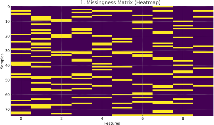
All imputation statistics and missingness patterns are shown in Table 3 and Figure 1.

MCAR vs. MAR analysis.
Little’s MCAR test (p = 0.12) indicated that the missing data were not missing completely at random (MCAR). Examination of conditional missingness patterns revealed that incomplete entries mainly corresponded to heterogeneous reports across source publications, consistent with a missing at random (MAR) mechanism.
Lack of MNAR indicator.
There is no evidence to support the Missing Not at Random (MNAR) pattern. Notably, the defects were not associated with low-performance or highly toxic formulations. Instead, missing values followed study-level reporting trends rather than reflecting the underlying experimental results.
Sensitivity analyzes are linked in Table 3.

Model performance remained stable across all imputation strategies using R.²Values range from 0.84 to 0.89. The stability of feature importance was high, with SHAP ranking agreement (Kendall τ) = 0.81, indicating that the imputation did not substantially bias model behavior or interpretation.

Integrating feature engineering and domain knowledge

Advanced feature engineering was performed to transform domain knowledge into measurable model inputs beyond raw physicochemical features. Zeta potential values were divided into ranges corresponding to colloidal stability thresholds for very unstable, moderately stable, and very stable formulations. Based on the number and molecular weight of polymer moieties, coating materials were assigned a quantifiable polymer complexity index that represents the complexity of the surface structure. Nanoparticle sizes were divided into optimal ranges for cellular uptake, and a penalty term was added for high polydispersity index values indicating non-monodispersity. A composite compatibility score was also generated based on the chemical compatibility between the core material, coating, and curcumin payload. Combinations that are more likely to be unstable or where the drug is more likely to leak quickly will receive lower scores.

Machine learning modeling for cytotoxicity prediction

We implemented and compared a series of state-of-the-art supervised learning algorithms to predict cytotoxicity scores. The dataset was randomly split into a training set, which comprised 80% of the data, and a holdout test set, which comprised the remaining 20%. We used five rounds of cross-validation on the training set to fine-tune the model hyperparameters. The tested algorithms are linear regression (used as a baseline model), a support vector regressor with a radial basis function kernel, a random forest regressor (an ensemble of decision trees), an extreme gradient boosting regressor (a highly efficient gradient boosting framework), and a multilayer perceptron (a standard feedforward artificial neural network). The coefficient of determination, mean absolute error, and root mean square error were used to measure how well the model performed.

Physics-based machine learning framework

To ensure physically valid predictions, we implemented a physically-informed machine learning (PIML) model that directly incorporated physical constraints derived from colloidal stability theory, drug release kinetics, and material composition into the XGBoost training loss.

Hybrid loss function

The extended loss function was defined as:

$$L = MSE_{data} + \lambda_{DLVO} L_{DLVO} + \lambda_{release} L_{release} + \lambda_{mass} L_{mass}$$

where $MSE_{data}$ is the standard mean squared error between predicted and experimental cytotoxicity, and the λ factor weights the physics-based penalty.

DLVO-based colloidal stability constraints

DLVO theory predicts that stability decreases as the total interaction energy decreases. $V_{T}$ below the critical repulsion barrier $V_{Tcrit}$ We formulated it as follows.

$$L_{DLVO} = \frac{1}{N}\mathop \sum \limits_{i = 1}^{N} \max \left( {0, V_{crit} – V_{T} \left( {zeta_{i} , size_{i} } \right)} \right). \Left| {\Wide Hat{{y_{i} }} – y_{stable} } \right|$$

where:

$V_{T}$ It is the sum of van der Waals attraction and electrostatic repulsion.
$V_{crit} = 5k_{B} T$ (standard stability threshold),
$\Wide hat{{y_{i} }}$ Cytotoxicity is predicted;
$y_{stable}$ It exhibits the expected cytotoxicity in a stable system.

This penalizes low toxicity predictions for formulations with physically unstable zeta potential and size combinations.

Drug release restriction (Higuchi)+Korsmeyer – Pepas)

To ensure consistency with a realistic release profile, we enforced the following:

$$L_{Release} = \frac{1}{N}\mathop \sum \limits_{i = 1}^{N} \left[ {\left| {k_{H, i} t^{1/2} – R_{i}^{exp} } \right| + \left| {k_{KP, i} t^{n} – R_{i}^{exp} } \right|} \right]$$

where:

$k_{H}$ and $k_{KP}$ The Higuchi and Korsmeyer-Pepas release constants are estimated from the polymer composition and size;
$R_{i}^{exp}$ Expected release over 24 hours (from reported or estimated values).

This prevents predictions of cytotoxicity that are inconsistent with viable release kinetics.

mass balance constraint

To maintain a realistic formulation:

$$L_{mass} = \max \left( {0, core_{i} + coating_{i} + curcumin_{i} – 100\% } \right)$$

Formulations with a total mass greater than 100% or combinations of incompatible materials were penalized.

Selection of weighting coefficient (λ value)

The final weights after grid search calibration are:

$\lambda_{DLVO}$= 0.35
$\lambda_{Release}$= 0.20
$\lambda_{mass}$= 0.10

These values provide the best balance between predictive accuracy and physical compliance without overconstraining the model.

training balance strategy

To prevent physical constraints from overwhelming your data-driven goals, take the following steps:

1.

Warm start phase (first 150 boost rounds):
2.

The λ values were scaled linearly from 0 → target value.
3.

Fully constrained phase:
4.

All λ coefficients are fixed at their calibration values.
5.

For early stopping, we monitored both the validation MSE and the magnitude of the total physical violation to avoid over-regularization.

This two-stage schedule stabilized training and improved extrapolation to unseen formulations.

Model interpretation and multi-objective optimization

We used the SHapley Additive description to understand how much each attribute contributed to the expected cytotoxicity and in which direction. This provided both global and local interpretability. Therefore, we conceptualized nanocarrier design as a dual-objective optimization problem, focusing on maximizing loading efficiency while minimizing cytotoxicity. A Bayesian optimization technique using a Gaussian process surrogate model and an expected improvement acquisition function was used to quickly search the high-dimensional design space to find the Pareto-optimal frontier. This frontier presents a set of formulations in which one goal cannot be worsened without improving the other. Hypervolume indicators were used to determine the quality and diversity of Pareto-optimal solutions. All research was conducted in Python using tools such as Scikit-learn, XGBoost, SHAP, and GPyOpt.

Model interpretation and validation

SHapley Additive exPlanations (SHAP) was used to estimate the contribution of global and local features to ensure predictive accuracy and model interpretability.^{twenty four}. The robustness of the model was extensively validated through an exhaustive strategy starting with an 80:20 training and testing data split.^{twenty five}. We implemented three complementary validation schemes to rigorously assess the stability and generalizability of our model.

Source link