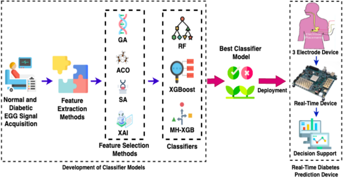
The proposed framework is categorized into two different parts namely development of best classifier models and deployment of developed classifier model into a real-time diabetes monitoring device. Figure 1 illustrates the proposed framework architecture for differentiating normal and diabetic affected EGG signals.

Scenario diagram of the proposed framework.
Firstly, the EGG signals are recorded from two sets of people, such as normal individuals and people suffering from diabetes. Once the EGG signals are acquired, the time and frequency domain features are extracted from the acquired signals. Further, the significant features are selected using various feature selection methods such as Genetic Algorithm (GA), Ant Colony Optimization (ACO), Simulated Annealing (SA) and SHAP based Explainable AI selection methods. Also, these features are fed to various classifiers and the performance of the various classifier models namely Random Forest (RF) Classifier, Extreme Gradient Boosting (XGBoost) classifier, Meta-Heuristic based Hybrid Extreme Gradient (MH-XGB) Boost Classifier are analyzed. Then the best classification model is used for categorizing normal and diabetic disorders, based on the performance metrics estimated from the EGG signals. Finally, the best classification model is deployed in portable real-time diabetes health monitoring device.
Development of classifier models
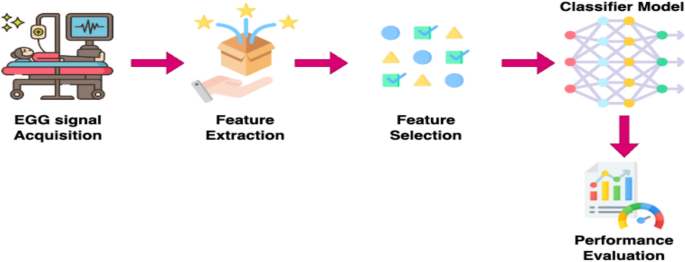
The development of classification models includes EGG signal acquisition, feature extraction methods, feature selection methods and development of machine learning models for classification. Figure 2 presents the block diagram of classification models development (The authors would like to clarify that the images (2, 3 and 4) in the manuscript were drawn using “drawio” open source online platform (https://www.drawio.com/).

Block diagram of classification models development.
An EGG signal acquisition involves the acquisition of EGG signals from normal individuals and patients suffering from type-II diabetes. Further, the possible features are extracted from the acquired EGG signals with the help of various time domain and frequency domain feature methods. Once the features are extracted, the prominent features are selected using selection methods which shall improve the performance of the classification models. In the final step, selected features are given as input to various classification models including proposed model and performance of the classification models are analyzed to identify a best classifier model.
EGG signal acquisition and pre-processing
A three-electrode portable EGG signal acquisition device is designed and developed in the proposed work, to acquire EGG signals from normal individuals and people suffering with type-II diabetes13. Further, the surface electrodes are utilized to acquire EGG signals which results in non-invasive EGG signal acquisition. Also, the standard placement protocol of three electrode systems is adopted and the proper written consent has been obtained from all the participants included in this study. Additionally, the study is reviewed and approved by the Institutional Ethics Committee at Gleneagles Global Health City, with the approval number (BMHR/2023/0055). The non-invasive electrodes are arranged based on a standard electrode placement protocol22. EGG signals acquired in the form of time in seconds and amplitude in volts are stored in the Comma Separated Value (.csv) file for further analysis. The EGG signals from 120 participants, namely 60 normal individuals and 60 persons with type-II diabetes are acquired and the EGG signal database has been created. Similar to denoising of Electrocardiogram (ECG) signals, the denoising of EGG signals are essential23. The pre-processing/denoising of acquired EGG signals are done by Empirical Mode Decomposition (EMD) which decomposes the acquired EGG signal into various frequency components called as Intrinsic Mode Functions (IMFs). The extraction of number of IMFs depends on two basic requirements namely the total number of zero-crossings/extrema should be similar or differ by at most 1 and the value of IMFs should be 0 for the mean of upper and lower envelopes. By using EMD algorithm, the EGG signal y[n]) can be given as follows24:
$$y\left[ n \right] = \mathop \sum \limits_{i = 1}^{k} IMF_{i} \left[ n \right] + p_{k} \left[ n \right]$$
(1)
where IMFi[n] is the ith IMF and the pk[n] is the residue. Also, the k represents total number of IMFs. Furthermore, the number of IMFs to be generated is determined by various factors such as length, nonlinearity and nonstationary of the EGG signals. Additionally, the IMFs exhibiting the ultra-low frequency components and power line interference less than 1 Cycles Per Minute (CPM) and beyond 20 CPM respectively were removed. Furthermore, the rest of the IMFs were added results in filtered EGG signal.
Feature extraction methodologies
A total of twenty features are considered for the proposed work, from two different domains namely time and frequency, are extracted from both normal and diabetic EGG signals. Further, the 17 different time domain features such as Variance (V), Root Mean Square (RMS), Mean Absolute Value (MAV), Maximum Fractal Length (MFL), Skewness, Waveform Length (WL), Teiger Kaiser Energy (TKE), Renyi and Tsallis Entropy (with five different orders) are extracted from the normal and diabetic EGG signals.
Variance (V) is a statistical estimation of a difference in values among an array of a given EGG signal. Also, the variance is used to quantify EGG signal fluctuations and its role in distinguishing between different digestive activity patterns. More specifically, it expresses the deviation of each number in the signal to the mean values of the total numbers in the signal as stated in Eq. (2).
$$\sigma^{2} = \frac{{\sum {\left( {v_{1} – v_{2} } \right)}^{2} }}{N – 1}$$
(2)
where, Σ is the variance, v1 denotes the value of one observed value, v2 denotes the mean value of all observed data, and N represents the total observations.
RMS is used to infer the quality of a prediction. It finds the difference between actual and the predicted values. Then it generates the square root based on the mean values in order to find out the final result25. Maximum Fractal Length (MFL) is one of the important techniques used for measuring signals. It is used to measure the absolute value based on the signal length in terms of lowest scale. The Mean Absolute Value (MAV) is used to estimate the average set of magnitudes for the datasets considered26 as specified in Eq. (3).
$$MAV = \frac{1}{N}\mathop \sum \limits_{n = 1}^{m} \left| {x_{n} } \right|$$
(3)
where Q indicates the actual count of data available in the dataset, \(\left| {q_{n} } \right|\) denotes the absolute value of \(q_{n}\). Teager-Kaiser Energy (TKE), is used to calculate the signal’s energy at the specific moment for any type of waveforms (either continuous or discrete) in a specific time. This can also determine the signals in higher-order derivatives also, which is performed by the equation given below27 as given in Eq. (4).
$$TKE\left( t \right) = k\left( t \right)^{2} – k^{\prime}\left( t \right)k^{\prime\prime}\left( t \right)$$
(4)
Where k(n) indicates signal at time k, and k(n)′ is first order and k’'(n) are second order derivatives of k(n), respectively. For discrete-time signals, the formula is given in Eq. (5).
$$TKE\left( p \right) = k\left( p \right)^{2} – k\left( {p – 1} \right)k\left( {p + 1} \right)$$
(5)
where \(k(p – 1)\) and \(k(p + 1)\) are the adjacent samples to \(k(p)\). Entropy is the term used for measuring uncertainty in the given normal and diabetic EGG signal. Otherwise, the entropy is a measure of complexity of EGG signals which helps in identifying distinguishing patterns between normal and diabetic subjects. In general, there are various entropy methods such as Renyi, Tsallis, Shannon, etc.11. Renyi entropy for a certain order of \(\alpha\) is given in Eq. (6).
$$H_{\alpha } \left( {x_{i} } \right) = \frac{1}{1 – \alpha }\log \mathop \sum \limits_{i = 1}^{n} P_{xi}^{\alpha }$$
(6)
where xi is a possible value of X and \(P_{xi}\) is the probability of a random variable x. When the alpha value is equal to 1, it enters Shannon entropy. Also, when the alpha value increases, it gives more weight to the higher probability, and when the alpha decreases, it gives more weight to the lower probability.
For the order of q, the Tsallis entropy equation is given in Eq. (7).
$$H_{q} = \frac{1}{q – 1}\left( {1 – \mathop \sum \limits_{i = 1}^{n} (P_{xi} )^{q} } \right)$$
(7)
where xi are the possible values of X, \(P_{xi}\) is the probability of xi, and n is the number of distinct values of X. Waveform length (WL) is an aggregate of waves along the region as stated in Eq. (8). Further, it determines the frequency, amplitude, and period of the EGG signals28.
$$WL = \mathop \sum \limits_{n = 1}^{N} \left| {x_{i} – x_{{\left( {i – 1} \right)}} } \right|$$
(8)
Skewness indicates the asymmetrical distribution of the collected EGG signals as given in Eq. (9). Depending on the extension of its tail it can be positive or negative. Skewness values tend to be zero when the distribution of the tail is symmetric29.
$$\gamma = E\frac{{\left( {x – \mu } \right)}}{{\sigma^{3} }}^{3} = \frac{{\mu^{3} }}{{\sigma^{3} }}$$
(9)
where E denotes expectation operator, \(\sigma\) denotes standard deviation, x denotes mean and \(\mu\) denotes mode of the signals.
The three different frequency domain-based features (Spectral Entropy, Frequency of Mean and Frequency of Median) are extracted from normal and diabetic EGG signals30. Spectral entropy is a method to quantify the randomness of a signal frequency as given in Eq. (10). Fourier Transform is used for converting the time domain to frequency domain31.
$$H = – \mathop \sum \limits_{n = 1}^{m} P_{n} {\text{log}}\left( {P_{n} } \right)$$
(10)
where P is the probability power of nth frequency, and m is the total spectral lines. The mean frequency is used in signal processing which analyzes the characteristics of the signal. There are different methods to calculate the mean frequency. Mean frequency is calculated by Power spectral density. The median frequency method is used for finding signal present in the spectrum’s central frequency. Mathematically it can be expressed as frequency of total sum of power spectral density divided by 2. This yields 50% of the total signals.
Feature selection methods
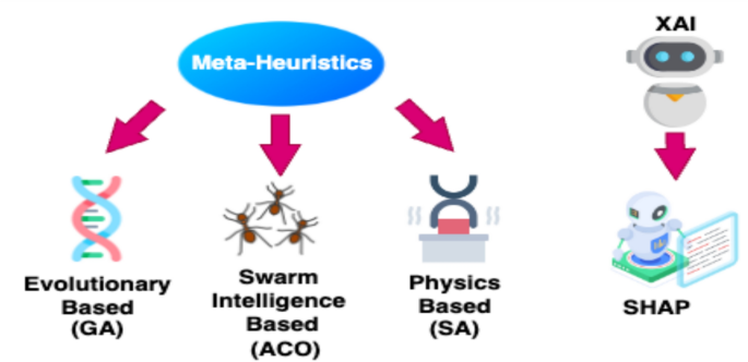
Figure 3 shows Meta-Heuristics and XAI based feature selection techniques utilized in the proposed framework. Furthermore, three different Meta-Heuristics based feature selection methods such as GA, ACO and SA are used for feature selection process. The GA ensures diversity and adaptability, ACO provides robust global search capabilities, SA offers energy-efficient and well-balanced exploration. However, the proposed Meta-Heuristics based feature selection methods were chosen to reduce computation time, improve accuracy and enhance model interpretability by selecting the most relevant features efficiently.

Meta-Heuristics and XAI based feature selection methods.
Also, an Explainable AI based feature selection method namely SHapley Additive exPlanations (SHAP) is utilized for the selection of prominent features from the acquired normal and diabetic EGG signals. Generally, the SHAP provides feature importance in EGG classification using following steps:
Step 1: Extraction of EGG signal features
Step 2: Training the MH-XGB classifier
Step 3 (Computing SHAP Values): SHAP assigns an importance score to every feature extracted from EGG signals which explains its contribution towards classification. If the SHAP value is positive, then the feature increases the likelihood of a class whereas the SHAP value is negative, then the feature reduces the likelihood of a class.
Step 4 (Visualizing SHAP explanations): SHAP displays global feature importance across all EGG signals.
The feature selection methods such as SHAP-based XAI and meta-heuristics are employed however, the Recursive Feature Elimination (RFE) or Principal Component Analysis (PCA) has following limitations.
-
The original features are transformed into new uncorrelated dimensions by PCA makes interpretation more difficult whereas the SHAP ranks the original features by importance.
-
Using RFE, the features are recursively eliminated by retraining the model multiple times resulting in not suitable for high-dimensional datasets.
The strategy of feature selection plays an important role in machine learning models for decreasing the complexity32, which in turn improves the performance of the proposed model.
Classification of EGG signals based on ML classifiers
The three different Classifier models namely Random Forest Classifier, Extreme Gradient Boosting (XGBoost), Meta-Heuristic based Hybrid Extreme Gradient (XG) Boost Classifier are utilized to classify normal and diabetic EGG signals obtained from normal and persons with Type-II diabetes respectively.
-
(a)
Random Forest Classifier:
Random forest algorithm is the most commonly used machine learning strategy. The RF method is much preferable because of its versatile features, including classifying and averaging, selection of subsets, accuracy, decision trees, and bagging methods. Also, the RF method overcomes the difficulties of overloading the data and has compared to the other learning algorithms, random forest is quite complex to visualize but provides accurate precision values33.
-
(b)
XGBoost and proposed MH-XGB Classifier:
The boosting family of algorithms comprises Category Boosting (CatBoost), Light Gradient Boosted Machine (LightGBM), and eXtreme gradient boosting (XGBoost). XGBoost is based on supervised learning by labeling the parameters and classifying them33. Extreme gradient boosting method is one of the effective algorithms in machine learning. Also, it includes the performance of the random forest and archives for better accuracy. XGBoost is more flexible, reduces the bias variables, and optimizes the assembler functions. XGBoost model is otherwise termed as an ensemble model which comprises of various weak classifier models into a strong classifier model. Generally, the XGBoost classifier model uses gradient boosting framework in which the model training is optimized by adding new trees iteratively with respect to residuals of the previous iterations. For a faster training process, XGBoost integrates and utilizes a hardware tool, namely a Graphics Processing Unit (GPU) processing power. There are various parameters and hyperparameters are applied to XGBoost to enhance the learning rate. Parameters customarily learn the data values, whereas in hyperparameters, the values are assigned manually and trained. Some of the parameters used by XGBoost are discussed below.
-
n_estimators:
The decision tree count is set by the n_estimators. The performance can be increased by increasing the number of trees, which also increases the programmable cost.
-
eta (learning rate):
In order to overcome over fitting the values, step size reduction technique is employed in modification. The weights of new features are updated by the boosting step. Also, the eta ranges from [0, 1]. Preferably, values are selected between 0.01 and 0.3.
-
max_depth:
It indicates the maximum depth of a tree, and it ranges from 0 to infinity. Also, the algorithm’s complexity depends on the depth of the tree.
The Eqs. (11–14) is utilized for the aforementioned process.
$${\text{Gain}} = \left( {{\text{S}}_{{\text{r}}} – {\text{ S}}_{{\text{l}}} } \right) – {\text{ S}}_{{{\text{root}}}}$$
(11)
$${\text{S}} = \frac{{\left( {\text{Sum of residuals}} \right){* }\left( {\text{Sum of residuals}} \right)}}{{{\text{No of residual}} + {{ \gamma }}}}$$
(12)
$${\text{Y}} = \frac{{\left( {\text{Sum of residuals}} \right)}}{{{\text{No of residual}} + {{ \gamma }}}}$$
(13)
$$Prediction = Base score + n.\left( {T_{r1} + T_{r2} + \cdots + T_{rn} } \right)$$
(14)
where Sr is right node similarity score, Sl is left node similarity score, Sroot is root node similarity score, \(\gamma\) is a parameter for regularization, y is the output at the leaf node, n is the learning rate, Tri is the leaf node output from the ith tree. Also, the residual is the difference between actual value and predicted value.
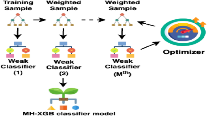
Figure 4 depicts the functionality of MH-XGB classifier model. The proposed MH-XGB classifier model is a combination of XGBoost classifier model with the meta-heuristic optimizer. The hyper parameters of the XGBoost classifier such as n_estimators, learning rate and max_depth are optimized using meta-heuristic optimizer. Further, the proposed MH-XGB classifier adapts Grey Wolf Optimization (GWO) as a meta-heuristic. In traditional GWO, the wolf attacks its prey by following the sequence of searching, judging and encircling the prey. In MH-XGB, the hyper-parameters are chosen by following a sequence of searching and identifying among the available parameter set, then choosing specific parameters based on estimation and then improving the same.

Design and functionality of MH-XGB classifier model.
The performance of the MH-XGB classifier model is continuously monitored and the hyper-parameters are adjusted by the optimizer, which in turn ensures the better performance when compared to the existing XGB. Also, the proposed MH-XGB classifier is superior over other classifiers because it selects the prominent/most relevant features and optimizes hyperparameters with the help of meta-heuristics which leads to improved accuracy and efficiency. Moreover, the proposed MH-XGB classifier outperforms Random Forest Classifier by reducing feature redundancy. Furthermore, the MH-XGB classifier uses a gradient boosting framework instead of independent trees results in improved generalization. Table 1 presents the comparison of MH-XGB classifier with RF and XGBoost in terms of strengths, weaknesses, and specific application benefits.
Real-time digestive health monitoring device
A MultiProcessor System on Chip (MPSoC) ZCU 104 evaluation kit is utilized to deploy the best classifier model and the efficacy of the model is analyzed. The ZCU104 has a quad-core ARM Cortex A53 processor and a real-time processor with dual-core Cortex-R5. Further, it has a graphics processing unit, namely Mali™ -400 MP2.
The three electrode EGG acquisition device is connected to the ZCU104 evaluation kit. Further, the best classification model is deployed into the ZCU104 evaluation kit. In common, there are two different ways in which the classification model shall be deployed into ZCU104 evaluation kit namely Vivado Design Suite and Jupyter Notebook. In this work, the classification algorithm is programmed using the Python programming language and is executed using a Jupyter notebook. However, python programming was utilized to develop MH-XGB classifier model and the deployment into ZCU104 evaluation board, the Vivado design suite shall be utilized in the near future to synthesis chip level fabrication which exhibits various advantages such as less memory, low power consumption and less size occupation.


