Explanation of experimental data
In this paper, we make use of the commonly used CICIDS2017 dataset.29As a widely accepted benchmark, CICIDS2017 shows good applicability30 It has been widely used in research into various network anomaly detection methods.31The dataset provider offers both the original pcap files and preprocessed versions containing 78 statistical features extracted using the CICFlowMeter tool, but in this paper we focus on processing the original pcap file data. The CICIDS2017 dataset consists of network traffic collected simulating real-world attack scenarios over a five-day period, from Monday, July 3, 2017 to Friday, July 7, 2017. The Monday data consists of only regular network traffic, while the Tuesday to Friday data contains instances of DDOS, brute force FTP, and botnet attacks. The network traffic is precisely labeled based on the 5-tuple information of each flow.
Normal traffic and 10 types of attack traffic were extracted from the original dataset as the test set and training set of the studied model. The data preprocessing process is described in detail. The final labels and corresponding quantities of the extracted data are shown in Table 5. From Table 5, we can see that the data samples labeled Normal and Port Scan far outnumber other samples. To prevent the imbalance in classification accuracy caused by too many samples of these two types of labels, during the octet classification experiment, these two types of samples were randomly undersampled, and 10,000 sample data were reserved for each type. In contrast, no undersampling was performed in binary classification.
The original traffic was preprocessed and converted into 1600-dimensional data. For visualization, the 1600-dimensional feature length was converted into a 40 × 40 matrix, and Figure 6 shows the grayscale maps of eight types of samples. From Figure 6, we can see that there are obvious differences between different samples. For example, in the Normal label and the Botnet label, it is easy to see that the textures are different between two samples, but there are also samples that are more similar. For example, two samples in the DDos label and the FTP-Parator label have only slight differences. In contrast, all samples of the same type show similar distributions between them, such as the Portscan label and the Web Attack label. In summary, there are large differences between samples of different labels, but samples of the same label have relatively similar textures.
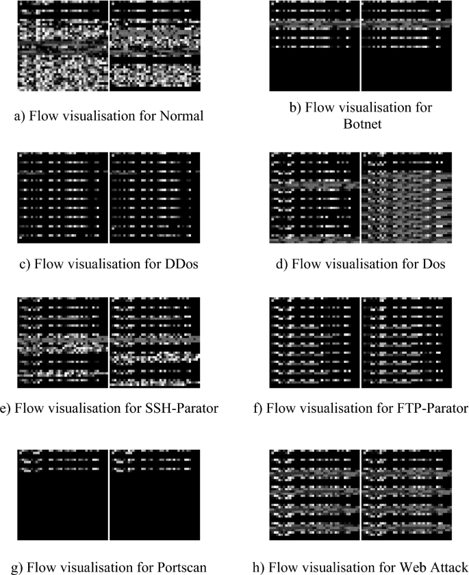
Visualization of eight samples from the CICIDS2017 dataset.
Analysis of experimental results
Accuracy, precision, recall, and F1 score are used as model performance evaluation metrics. Convolutional neural network models, AlexNet, ResNet, and some traditional machine learning models that use only raw traffic data were selected for binary and octet classification experiments. To ensure that all category samples are evenly distributed in the test and training sets, we select 70% of the total data from each label as the training set and 30% as the test set. The coding table of classification labels is shown in Table 6.
Determining model parameters
Some parameters of the convolutional neural network were experimentally tuned, and the performance of the model is highly dependent on the parameters of the neural network. First, we experimentally analyzed the number of convolutional channels to find the optimal number of convolutional channels. The number of convolutional channels in the first layer was set to 16, 32, 64, and 128, respectively, to compare the impact of the number of channels on the classification accuracy of the model while controlling other parameters constant. The experimental results are shown in Figure 7.

Classification results for different channel numbers.
From Figure 7, we can see that for binary classification, the classification accuracy gradually improves when the number of convolutional channels is 16, 32, and 64, and starts to decrease when the number of channels is 128. Also, when the number of channels is 64, the accuracy only improves by 0.01%, but the training time is longer. For octet classification, the number of channels already starts to decrease at 64. Therefore, considering performance and cost, the first layer was finally selected to have 32 channels in the proposed model.
Next, to compare the impact of different network layers of CNN on the performance of the model, we selected the number of convolutional layers from 1 to 4 and compared the accuracy while keeping other parameters constant. The experimental results are shown in Table 7.
As can be seen from Table 7, the model with one convolution layer has the worst performance. In binary classification, the performance of three convolution layers is slightly better than that of two convolution layers, but the model accuracy begins to decrease when the number of layers reaches four. In multiple classification, the model accuracy already begins to decrease with three convolution layers. Although the three-layer model performs somewhat better in terms of binary classification, the deeper the layers, the more parameters there are and the higher the learning cost. Considering both performance and cost, we finally chose a two-layer convolution neural network model as the layer in this paper.
Finally, to investigate the impact of 1D and 2D convolution on the model performance, we also tested the difference in classification accuracy of models in octet classification for different layers of 1D and 2D convolution.
From Table 8, we can see that the classification accuracy of the 2D convolutional model at any number of layers is lower than that of the 1D convolutional neural network model.
Binary Classification Experiments
The classification results of this paper on the CICIDS2017 dataset using classical machine learning models such as CNN and random forest are shown in Table 9. The CNN model applied in this paper, this CNN1D model, uses one-dimensional convolution to extract features directly from raw traffic without combining statistical features compressed by an autoencoder. As can be seen from Table 9, when performing binary classification on the CICIDS2017 dataset, deep learning models generally outperformed traditional machine learning models, all achieving accuracy above 99%. Also, the model proposed in this paper performed the best among all models, reaching the highest values in all four metrics. SVM was the worst performing model.
Multiple classification experiments
To further verify the performance of the model, an experimental study of octet classification was conducted on the CICIDS2017 dataset. The experimental results of octet classification are shown in Table 10. From Table 10, we can see that the performance of the three deep learning models, AlexNet, ResNet, and CNN1D, still outperforms traditional machine learning models in octet classification. Meanwhile, we can see that among the traditional machine learning models, KNN performed the worst. The proposed model achieved an accuracy of 98.51%, a precision of 98.31%, and an F1 score of 98.31%, which were the best among all models with the highest values.
To clearly show how accurately the model predicted the samples for each class, we plotted the confusion matrix shown in Figure 8. As can be seen from Figure 8, we were able to correctly classify most of the samples. Most of the incorrectly predicted samples with label 4 were predicted to sample 5. As can be seen from the gray scale plot, there are indeed many similarities between the two labeled samples, which can make classification difficult for the model and lead to misclassification of the model.

Confusion matrix for the CICIDS2017 dataset.
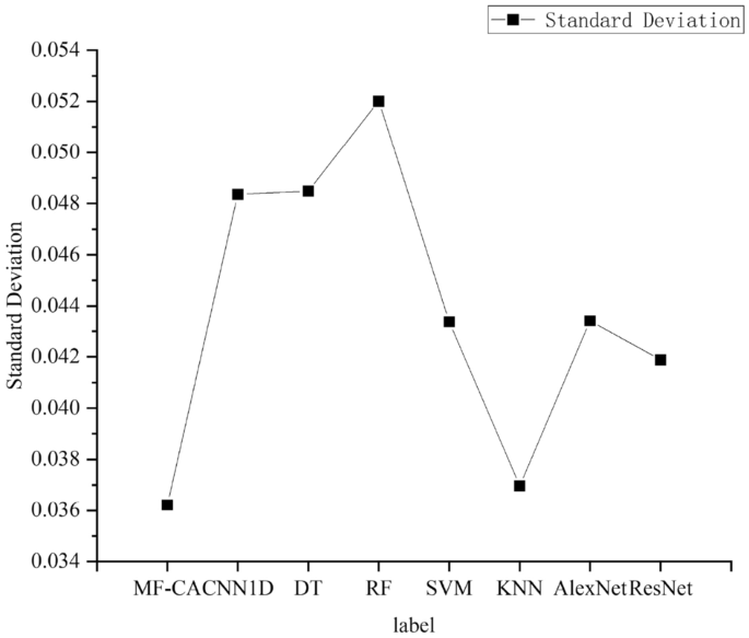
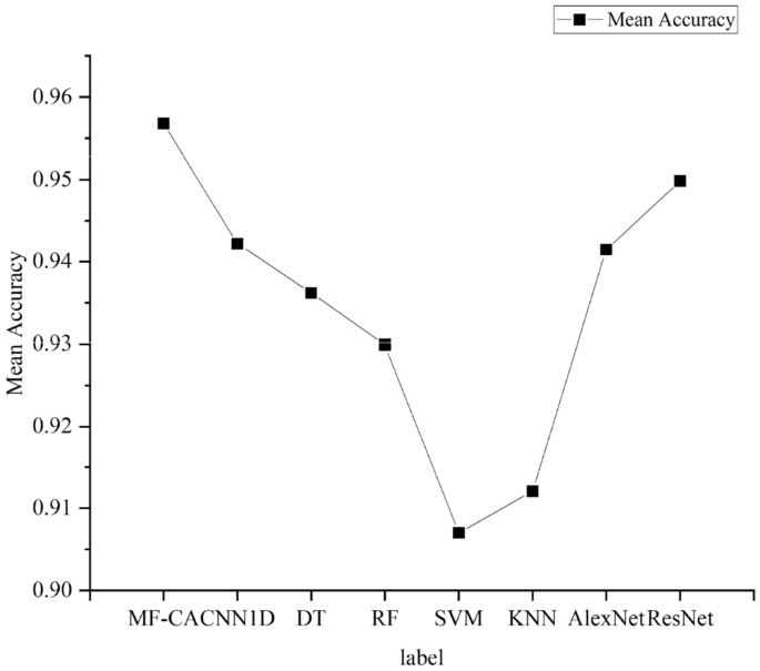
To compare the classification performance of the models on different types, we plotted the F1 scores of the models on each category. As shown in Figure 9, the graph shows that the proposed model achieves the highest F1 scores on most labels and has the best overall performance. To facilitate the analysis of the test performance of the algorithm proposed in this paper, additional statistical analysis was conducted. The standard deviation and average accuracy are shown in Figures 10 and 11, respectively. It is worth noting that the algorithm proposed in this paper achieves the smallest standard deviation and the highest average accuracy, indicating its excellent robustness and generalization ability.

Comparison of F1 scores in each category for each model.