
Dataset collection
Data collection and acquisition are the primary steps in creating any ML model. It comprises a literature study or a direct experimental assessment of pharmacological substances and their inhibitory effects29. A dataset from the publicly accessible Binding database was used in this investigation. The collected GSK3β dataset includes 4087 chemicals tested against GSK3β in a laboratory and had known biological activity (IC50 values). After filtering the compounds of interest, a three-column SAR file was produced. The BindingDB ID, which identifies a molecule and its function, is in the first column. The compound’s molecular structure is examined by looking at its SMILES format in the second column. The pIC50 values in the third column have been meticulously collected from scientific literature. Measurements were made in nM, mM, and mM/mL. Any units not in nM must be changed to nM to normalize these data. It was then converted to its negative logarithm form, pIC50, for the same size. We used these three pieces of information in the SAR dataset to create several ML classification and regression models30.
Generation of molecular descriptors
The chemical, physical, and structural characteristics of molecules are quantified and encoded into numerical form by molecular descriptors. These descriptors provide the basis for computational models that predict biological activities for new drugs, including Quantitative Structure–Activity Relationship (QSAR), Structure–Activity Relationship (SAR) and Virtual Screening (VS) assessments.
Using Python (v3.9) and the MORDRED algorithm, a total of 1826 (1D, 2D, and 3D) molecular descriptors were calculated for 4087 molecules in this study. MORDRED was implemented using the cheminformatics framework RDKit for converting and parsing chemical structures. Topological, constitutional, autocorrelation, geometrical, electronic, and steric characteristics were among the descriptors that were produced. A Python pipeline that included tools like Joblib for parallel processing and NumPy and Pandas for matrix manipulation was used to automate the descriptor computation technique. Before descriptor extraction, all compounds were standardised in SMILES format and optimised using the MMFF94 force field to improve computational performance and guarantee descriptor repeatability. After exporting the final descriptor matrix in CSV format, it was prepared for additional preprocessing and model construction using ML methods as Random tree, Decision Table (DT), Random Forest (RF), KStar and Instance-Based K-Nearest neighbours (IBK)31.
Data pre-processing
Overfitting and worse prediction performance can result from the presence of duplicated, unnecessary, or noisy features in a raw descriptor matrix. Consequently, in order to guarantee high-quality input for ML modelling, thorough data pretreatment was taken. Using the Scikit-learn, NumPy and Pandas frameworks, the workflow was mostly developed in Python and comprised data cleansing, dimensionality reduction, outlier identification and feature scaling32.
Data cleaning
Incomplete or missing data may make the model less accurate. The Pandas isnull () and dropna () methods were used to identify and then delete rows that included empty cells, NULL, or NaN values. 744 valid molecular observations that were prepared for additional investigation were obtained after 1083 incomplete records were eliminated33.
Dimensionality reduction
A model’s prediction ability may increase as the number of features increases. Still, eventually, the model’s performance may decline due to a phenomenon known as the “curse of dimensionality”. To build a powerful ML model, dimensionality reduction reduces high-dimensional data into lower dimensions. Eliminating superfluous features from the dataset al.so simplifies the model. Using the feature selection and NumPy modules from Scikit-learn, the preprocessing pipeline comprises the following sequential filters34. The reduced descriptors are shown in Table 1, and to ensure the descriptor reduction, a Heatmap was generated as given in Fig. 1.
Constant filter
Specific descriptors had zero variance and provided no valuable information for model predictions since they were consistent across all samples. These constant characteristics were eliminated using a variance threshold filter set to zero. As a result, there were 612 descriptions instead of 74435.
Low variance filter
Additionally, quasi-constant characteristics having more than 99% identical values did not significantly improve prediction accuracy. Nearly negligible variance was seen in these characteristics. With a variance cut-off of 0.011, a low-variance filter was used to solve this. The descriptor count was further decreased from 612 to 540 as a result36.
High correlation filter
Finding descriptors that have a strong correlation with one another aids in removing duplicate characteristics. Ensuring that just one of the linked features is kept decreases the model’s dimensionality and avoids needless complexity. Pearson’s Correlation Coefficient (r) is the most often used correlation metric; it measures the linear connection between two variables. Pearson’s correlation formula is given below37.
$$\:r = \frac{{\sum \: _{{i = 1}}^{n} \left( {x_{i} – x^{ – } } \right)\left( {y_{i} – y\:^{ – } } \right)}}{{\sqrt {\sum \: _{{i = 1}}^{n} \left( {x_{i} – x^{ – } \:} \right)^{2} \left( {y_{i} – y^{ – } } \right)^{2} } }}$$
Were,
r is the correlation coefficient,
xi are the x value, x̄ is the mean of the x values,
yi are the y values, and ȳ is the mean of the y values.
The Corr function was used to calculate the correlation values between the 990 descriptors. Only one descriptor was kept if the correlation coefficient between any two of them was higher than 0.75. Through this technique, there were 243 descriptors instead of 540 characteristics. Before and after this filter was applied, feature association was shown using a heat map display.
Outlier detection and removal
Outliers are extraordinary data points that deviate from the dataset’s general trend. They could harm ML algorithms. We used the following formula for the remaining 243 observations to determine the Z-scores: An outlier was identified and removed for each observation with a Z-score greater than 7 by using SciPy stats.zscore function. This means the sample size was reduced to 190 observations after 53 outliers were eliminated38.
$$\:Zscore\: = \frac{{x – \mu \:}}{{\delta \:}}$$
The variable’s mean is µ, while the standard deviation is δ.
Scaling of molecular descriptors
Following pre-selection, the entire dataset was normalized to the same range using the min-max normalization using Scikit-learn’s MinMaxScaler, which scales all the molecular descriptors information between 0 and 1. It is calculated by dividing the difference between the highest and lowest values in a column by the difference between any value and the lowest value. Scaling ensures that every descriptor plays an equal part in building the prediction model and allows for the accurate comparison of several ML models. Usually, this is completed before using the attributes to create the model39.
$$\:X\:normalization = \frac{{x – x_{{\min }} }}{{X_{{\max }} – x_{{\min }} }}$$
Where x is the individual X values, Xmax and Xmin are the maximum and minimum values.
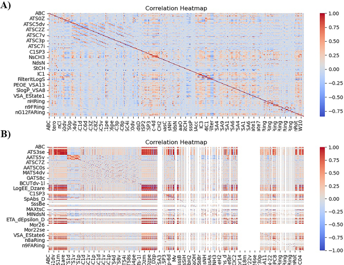
Heat map representation of before and after removing correlated features.
Selection of training and test set
Following the removal of the most relevant characteristics, the 4087 observations in the data were randomly split into the train and test sets. The ML model is trained using the training set containing 70% of the data. The built model is tested using the test set, which includes 30% of the remaining data. For the target variable, 2861 molecules were employed in the train set and 1226 in the test set.
ML methods
To build a variety of ML models for forecasting the biological activities of new compounds, this study used six supervised ML algorithms: Random Forest (RF), Decision Table (DT), Random Tree (RT), Instance-Based K-Nearest Neighbours (IBK), KStar (K*), and Locally Weighted Learning (LWL). Table 2 provides a summary of the chosen supervised learning models40,41,42.
Random forest (RF)
RF is a supervised learning approach that generates several decision trees by bootstrap data sampling and random feature selection at each split. Each decision tree provides a vote (for classification) or an averaged value (for regression), and the aggregate result is more reliable and accurate than a single tree. The main goal of Random Forest is to average over a large number of subpar learners to reduce volatility and decrease bias43. This enables it to effectively handle missing values, noisy data, and high-dimensional datasets. It also provides an understanding-facilitating feature relevance metric. It has been widely employed due to its high predictive performance in several domains, such as finance and biology, and its ability to generalize effectively with minimal parameter change44.
Decision table (DT)
The model is easy to use and comprehend since each row denotes a rule that specifies an output based on specific combinations of input attributes45. In situations where accountability, transparency, and conformity are necessary, such as in regulatory or medical applications, statistical black-box models are less efficient than decision tables. Because the technique accurately translates attributes to decisions without requiring complex transformations, stakeholders who are not technical may understand model behaviour. Despite their inferior predictive accuracy compared to modern ensemble techniques, decision tables might be helpful when interpretability is more important than raw performance46.
Random tree (RT)
Random Tree reduces the likelihood of determinant bias and enhances variation by restricting itself to a random selection of traits. A single Random Tree is the foundation of ensemble approaches like Random Forest, where merging several Random Trees yields potent prediction results, even though a single Random Tree typically has high variance and overfitting47.
Instance-Based K-nearest neighbours (IBK)
IBK is the WEKA variant of the k-nearest-neighbours (k-NN) algorithm, a well-liked instance-based or “lazy” learning method. IBK preserves all training instances and postpones computation until prediction time. When a new case has to be classified, the process finds the k closest cases to each stored example, calculates the distances (often Manhattan or Euclidean) to each one, and then guesses the label using a weighted scheme or majority vote. The main benefits of IBK are its simplicity and effectiveness, especially in domains where local patterns in data are very valuable48.
KStar (K*)
KStar, or K*, is an advanced instance-based classifier that extends the k-NN idea by including an entropy-based distance measure. KStar evaluates similarity by estimating the probability of transforming one instance into another through a series of stochastic transformations instead of relying solely on geometric distance measurements49. This method allows KStar to detect complex data connections that conventional distance measures would miss, increasing its versatility and effectiveness in specific domains. Its entropy-based reasoning can enhance classification performance and is robust to noisy features when Euclidean similarity measurements are subpar. KStar’s adaptability and ability to express non-linear or irregular similarity structures are the primary reasons for its usage in ML, even though it increases processing complexity50.
Locally weighted learning (LWL)
Locally Weighted Learning (LWL) is a lazy learning technique that does not develop a single global model but instead generates local models around a query instance. Regarding prediction time, it finds nearby data points, weights them according to how far away they are from the query, and then fits a basic model (such as Bayesian rules or linear regression) inside this limited area51. This technique allows LWL to identify non-linear, regional trends in the data that global models may miss. The flexibility of LWL is its greatest asset; it can adjust to changes in various dataset segments, which makes it useful for issues with diverse data distributions. It is less scalable to massive datasets and necessitates more processing at prediction time, just like other lazy learners. When localized modelling performs better than global approximation, its usage is warranted52.
Cross-validation
In the WEKA ML environment, 10-fold cross-validation was used to assess the regression model’s prediction performance. First, the entire dataset is randomly divided into 10 equal-sized subgroups, or “folds,” as part of this process53. The model is trained using nine folds, with the remaining fold being set aside for performance testing54. This procedure is performed 10 times in a sequence, using the remaining folds for training and presenting a different fold as the test set. To create a single overall performance estimate, the outcomes of every iteration are then averaged. The justification for utilizing 10-fold cross-validation is that, in contrast to a single train-test split, it can offer a more impartial and trustworthy evaluation of the model. This is particularly crucial for regression tasks, since the way the dataset is partitioned affects performance measures like Mean Absolute Error (MAE), Root Mean Squared Error (RMSE), Correlation Coefficient, and Relative Absolute Error (RAE). To do this, WEKA’s “Cross-validation” option was enabled with 10 folds in the “Classify” panel after choosing the regression technique of interest. WEKA carried out the ten training and testing iterations, automatically randomized the data, and provided the mean outcomes55. The values were computed as follows:
$$\:RMSE = \sqrt {\frac{{\sum \: _{{i = 1}}^{n} \left( {y_{i} – \hat{y}_{i} \:} \right)^{2} }}{n}}$$
$$\:MAE = \frac{{\sum \: _{{i = 1}}^{n} \left( {y_{i} – \hat{y}_{i} \:} \right)}}{n}$$
$$\:MSE = \frac{{\sum \: _{{i = 1}}^{n} \left( {y_{i} – \hat{y}_{i} \:} \right)}}{n}$$
$$\:R^{2} = \frac{{\sum \: _{{i = 1}}^{n} \left( {y_{i} – \hat{y}_{i} \:} \right)^{2} }}{{\sum \: _{{i = 1}}^{n} \left( {y_{i} – y^{ – } _{i} \:} \right)^{2} }}$$
Here,\(\:\:n\) represents the number of molecules, yi denotes the experimental value, ŷi the predicted value and ȳi the mean of experimental values.
Predictive ML model as a virtual screening
An ML-based regression modelling approach was employed to predict inhibitory activity and identify potential repurposable drugs for AD16. A curated dataset of experimentally reported inhibitors was used to train regression models for predicting the IC₅₀ values of compounds. The predictive performance of the models was validated using 10-fold cross-validation, and the most accurate regression model (based on statistical evaluators MSE, MAE, RMSE, and R²) was selected for further screening. A library (Drug Bank) of 4,099 FDA-approved drugs was retrieved for screening. Pre-processing steps were applied to ensure drug-like characteristics, including compound filtration (removal of duplicates, salts, inorganic molecules, and highly aliphatic compounds). After this step, 1,616 FDA compounds were retained. Descriptor generation and standardization were then performed, and the processed compounds were subjected to prediction using the trained regression model56.
Molecular docking
The FDA-approved compounds predicted by the regression model to exhibit inhibitory activity below 500 nM were selected for structure-based molecular docking57,58. The three-dimensional structure of the target protein (GSK3Beta) was retrieved from the Protein Data Bank (PDB ID: 8ff8) (https://www.rcsb.org/) and prepared by removing crystallographic water molecules and heteroatoms not involved in binding, adding hydrogens, and assigning appropriate protonation states. Ligand structures were obtained from Drug Bank, converted into 3D format, protonated at physiological pH, and energy-minimized using the MMFF94 force field. The prepared protein and ligands were converted into the AutoDock-compatible PDBQT format using AutoDock Tools with Gasteiger charges assigned. The active site was defined based on the co-crystallized ligand and literature-reported residues, and a grid box was generated with centre coordinates X = 19.51 Å, Y = −16.62 Å and Z = 79.26 Å and sufficient dimensions to cover the binding pocket. Docking simulations were performed using AutoDock Vina. The conformation with the lowest binding energy was selected for each ligand, and protein–ligand complexes were further analyzed using Discovery Studio Visualizer 2021, while the Schrodinger Maestro interface was employed to conduct the visualization and interaction analysis of the coupled complexes. Compounds with favourable docking scores and key binding interactions were prioritized as potential repurposable candidates for AD59.
Molecular dynamics simulation
The OPLS 2005 force field in the DESMOND v6.3 module of the Schrodinger suite was used to do molecular dynamics (MD) simulation tests on the chosen protein-ligand complexes from the molecular docking study. The protein-ligand combination was initially put within a cubic boundary box using TIP3 water as the solvent model to make the system builder. The protein was subjected to a second reduction and recalculation process to include additional counterions for charge balance inside the system60. To make the salt levels resemble those in the body, a solution with 0.15 M NaCl was added to the system 20 m away from the ligand. This protocol comprises nine stages, including two minimization steps and four short simulations (the equilibration phase) that happen before the true production period starts. The first molecular dynamics simulation investigations were done on the best-scoring ligand-receptor complexes, which ran for 10 ns. Second, 1000ns was utilized to find ligand-protein complexes that were highly stable so that they could be tested further61. We ran the simulations at 300 K and 1.01325 bar of air pressure, using the Optimized Potentials for Liquid Simulations (OPLS) 2005 force field and the NPT ensemble. We utilized the Simulation event analysis tool from the DESMOND module to look at the MD simulation results for complex RMSD (Root Mean Square Deviation), RMSF (Root Mean Square Fluctuations), Protein–Ligand interactions, and contacts with different amino acid residues62.
Absorption, distribution, metabolism, excretion and toxicity (ADMET) studies
ADMET studies are crucial in drug development, providing valuable information on a drug candidate’s pharmacokinetics and safety profile. ADMETlab 3.0 (Pharmacokinetics Chemistry, Small Molecule) is a computer program that uses ML to quickly guess ADMET characteristics. ADMETlab 3.0, which calculates the ADMET characteristics, utilizes SMILES of the ligand as its input format. ADMETlab 3.0 is particularly useful for improving drug discovery pipelines since it combines predictive models into one platform63.
Density functional theory (DFT)
The DFT has emerged as an effective tool for sensing and predicting the antidiabetic potential of molecules. DFT primarily aims to offer quantitative information about material properties by applying fundamental quantum mechanics concepts. This work used molecular docking to identify the top binding score active molecules, and computational measurements were carried out using the Gaussian 03 W software and the GaussView molecular visualization tool. The molecular structures of the discovered active molecule were optimized using Spartan. The optimized structures were utilized to calculate the frontier molecular orbital energies of the chosen bioactive chemicals. GaussView, a molecular visualization program, presented the molecular orbital energy diagrams for the selected bioactive molecules64.


