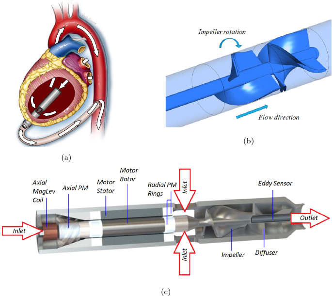
Figure 1a shows the proposed implant method for the NeoVAD, and although the specific speed, \(N_s = 1.762\) (operating at 15,000 rpm), of the proposed pump lies within the mixed-flow regime of a Cordier diagram25,26, size constraints limit the design to being an axial-flow device. The intended paediatric population is 5–20 kg. The target operating point for the smallest babies is a pressure head of 50 mmHg and flow rate 0.5 L/min while at the upper end of the range the target is 70 mmHg and 2 L/min. The initial target operating condition was the upper end of the scale and subsequently optimisation for the middle and low end of the scale was investigated.

(a) Implantation schematic of the NeoVAD in the left ventricle, (b) blade configuration inside the NeoVAD (image created in Ansys academic research CFX, release 21.1, https://www.ansys.com/products/fluids/ansys-cfx) (c) location of the blades inside the NeoVAD and other features including the MagLev motor and permanent magnets (PM) (image created in Dassault systèmes SOLIDWORKS 2020 https://www.3ds.com/products-services/solidworks/).
A typical blade setup for the NeoVAD is shown in Fig. 1b. Within this study, the naming convention is such that the rotating blade section is referred to as the impeller and the stationary section in referred to as the diffuser. The rotor-stator convention that is more common for axial-flow devices is avoided to reduce confusion with the magnetic levitation and motor parts that bear the same name. As can be seen from Fig. 1b the impeller consists of 2 rotating blades and the diffuser consists of 3 stationary blades, in keeping with the previous study by Smith et al.27. A cutaway view of the NeoVAD is shown in Fig. 1c. This view shows an overview of the NeoVAD highlighting the location of the impeller and diffuser blades, the motor rotor and motor stator, maglev bearing and associated permanent magnets, and inlets and outlet of blood flow.
Computational fluid dynamics
The blade geometry for this study is defined and parameterised in accordance with previous experiments27. The baseline design consists of an impeller of two blades and a diffuser of three blades. The blades themselves are of circular arc design and have a constant thickness of 0.5 mm and elliptical leading and trailing edges. Only the free parameters defined in previous experiments27 were considered for this study, such that each design simulation had an experimental counterpart, and to avoid introducing additional free parameters that could increase computational expense.

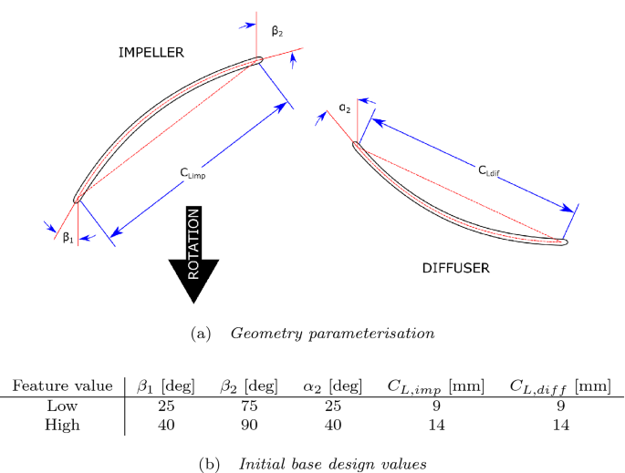
Parameterisation of the mid-span blade shapes into five governing parameters: impeller inlet angle, \(\beta _1\), impeller outlet angle, \(\beta _2\), diffuser inlet angle, \(\alpha _2\), impeller chord length, \(C_{L,imp}\) and diffuser chord length, \(C_{L,diff}\). Figure adapted from Smith et al.27.
Five variable parameters govern the blade shape as can be seen in Fig. 2a, namely the inlet angles and chord lengths of both impeller and diffuser blades and also the outlet angle of the impeller. The outlet angle of the diffuser is set to 90 degrees (as measured from the tangential direction) so as to align the downstream flow axially. Using this method, the camber line at mid-span can be calculated for any specified values of these five parameters.
Ansys®Academic Research BladeGen, Release 21.1 (Ansys Inc., Canonsburg, Pennsylvania, United States) was used to create the full impeller diffuser geometry by sweeping the profile between the hub, with a radius of 1 mm, to the shroud, with a radius of 3.85 mm. The full geometry was exported from BladeGen to Ansys®Academic Research TurboGrid, Release 21.1 (Ansys Inc.) where an impeller tip gap of 100 \(\mu\)m was added and a hexahedral mesh was created. The process, from specification of input parameters through to mesh creation was automated and controlled using a script created in MATLAB®R2020b (The MathWorks, Inc., Natick, Massachusetts, United States).
Smith et. al.27 used the parameterisation method shown here to create and test 32 different pump designs that consisted of 8 unique impellers and 4 unique diffusers. To do this, each of the 5 geometry-governing parameters was assigned a high and a low value, which can be seen in Fig. 2b. Combining these values in every configuration gives the 32 base designs.
Computational fluid dynamics simulation utilised Ansys®Academic Research CFX, Release 21.1 (Ansys Inc.) to solve either the Reynolds Averaged Navier Stokes (RANS) or unsteady RANS using a shear stress transport turbulence model, the SST k-\(\omega\). The flow field experiences a range of Reynolds numbers, with pipe flow based estimates in the inlet region spanning \(\text {Re} = {vD\rho }/{\mu } = 100 – 850\), where v is the average velocity based on the flow rate span of \(Q = 0.5 – 4\) L/min, D the diameter (7.7 mm), \(\rho\) the density (taken as 1050 kg/m\(^3\)28) and \(\mu\) the viscosity (taken as 0.0035 Pa\(\cdot\)s28). Using the rotor tip velocity for estimates in the rotating section, the Reynolds number can reach \(\text {Re} = {\omega D^2 \rho }/{\mu } = 37,000\), using an estimated maximum rotating speed, \(\omega = 20,000\) rpm. The total range of Reynolds number in the flow field puts this device in the transitional regime. The SST k-\(\omega\) model has been widely used in previous studies of rotary mechanical circulatory support devices28,29,30.
Fourth-order Rhie Chow pressure-velocity coupling was used and a blended spatial discretisation scheme that utilises second-order central differencing but using a blending function to introduce enough first-order upwind differencing to prevent overshoots when the local solution gradient is large31.
Mesh dependence
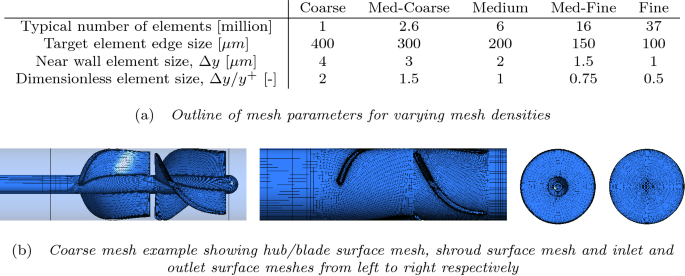
To explore the effect of the mesh density on the solution, a pump design was chosen at random from a list of 32 geometries that were studied experimentally. The default mesh density was set such that the first near wall elements were sufficiently small for a target of \(y^{+} < 1\). Other density meshes were created both coarser and finer such that solution comparisons could be made. Mesh parameters can be seen in Fig. 3a. Away from the wall, mesh element lengths were expanded smoothly and an example of the coarsest mesh can be seen in Fig. 3b.

Comparison of mesh creation parameters for mesh density study and an example mesh illustrating hexahedral element structure and expansion ratios.
Mesh dependency was evaluated for steady-state simulations utilising the mixing plane boundary method between the rotating and stationary frames of reference, which averages the pressure and velocity fields circumferentially at the reference frame boundary. Transient Unsteady RANS (URANS) and Detached Eddy Simulation (DES) simulations were also run for comparison, using the sliding plane boundary method, which conserves the pressure and velocity field across the boundary. In all instances the boundary is located at the midpoint between the impeller trailing edge and the diffuser leading edge. The transient simulations have a time-step length equivalent to \(5^\circ\) of rotation per time-step and run for 50 full rotations of the pump and the last 20 full rotations are averaged to find the pressure and efficiency results. Transient simulations are inherently more computationally expensive, and the mesh study allowed comparison of different density meshes but also a comparison of temporal solution methods.
Scaling
With designs that have been experimentally tested, the rotational speed required to pass through the given operating point of \(Q = 2\) L/min, \(H = 70\) mmHg has already been found. For designs to be simulated without prior knowledge of the required rotation speed, dimensional analysis was used. Simulations were carried out at an estimated speed (given that this estimate does not take the pump into an entirely different turbulence regime) and the resulting pressure-flow (HQ) and efficiency-flow (\(\eta Q\)) curves were scaled such that they fit the desired operating point. This gave the required rotating speed, that differed from the original estimate.
The 32 pump designs were simulated with a rotating speed of 20,000 rpm in the first instance. To scale the HQ curves such that they passed through the required operating point, a quartic polynomial was fit to the data, with the form
$$\begin{aligned} \Delta P = c_1 Q^4 + c_2 Q^3 + c_3 Q^2 + c_4 Q + c_5 \end{aligned}$$
(1)
The coefficients of this equation were found using MATLAB curve fitting tools.
Using the definition of the flow and pressure coefficients
$$\begin{aligned} \phi = \frac{Q}{\omega D^3}, \quad \psi =\frac{\Delta P}{\rho \omega ^2 D^2} \end{aligned}$$
(2)
it is possible to arrive at the similitude scaling laws between two operating points, which can be arranged such that
$$\begin{aligned} \Delta P_2 = \Delta P_1 \left( \frac{Q_2}{Q_1}\right) ^2 \end{aligned}$$
(3)
where the subscript 1 describes the desired operating point and subscript 2 describes the operating point on the resultant HQ curve at 20,000 rpm that shares the dimensionless coefficients, \(\phi\) and \(\psi\).
As the exact point on the resultant HQ curve that shares these dimensionless coefficients is unknown, we can substitute the quartic polynomial that describes the entire curve knowing that
$$\begin{aligned} \Delta P_2 = c_1 Q_2^4 + c_2 Q_2^3 + c_3 Q_2^2 + c_4 Q_2 + c_5. \end{aligned}$$
(4)
Equating Eqs. (3) and (4) and rearranging gives
$$\begin{aligned} c_1 Q_2^4 + c_2 Q_2^3 + \left( c_3 – \frac{\Delta P_1}{Q_1^2} \right) Q_2^2 + c_4 Q_2 + c_5 = 0 \end{aligned}$$
(5)
With the coefficients, \(c_{1 … 5}\) known, solving for \(Q_2\) allowed the calculation of \(P_2\) from the resultant HQ curve and subsequently the rotating speed \(\omega _1\) that resulted in the curve passing the desired operating point. Using the dimensionless coefficients of Eq. (2), the HQ curve and efficiency curve were rescaled.
Using this method, HQ and \(\eta Q\) curves can also be scaled to other operating points, namely \(OP_{1\textrm{L}/\textrm{min}}: \Delta P = 60\,\text {mmHg}, Q = 1\,\text {L/min}\) and \(OP_{0.5\textrm{L}/\textrm{min}}: \Delta P = 50\,\text {mmHg}, Q = 0.5\,\text {L/min}\). This allows the final optimised design—designed to maximise efficiency at \(OP_{2\textrm{L}/\textrm{min}}: \Delta P = 70\,\text {mmHg}, Q = 2\,\text {L/min}\)—to be evaluated for performance across a range of conditions expected throughout the development of a paediatric patient.
Surrogate model
Commonly implemented optimisation routines operate by regularly evaluating the underlying function. In the case of this study—optimising geometry for maximum efficiency—each function call would involve specifying the values of the five governing parameters, creating the geometry and mesh and running CFD simulations at multiple flow rates such that pressure- and efficiency-flow curves can be created. The former for scaling the results to the desired operating point and the latter for identifying the efficiency at the given design point of \(\Delta P =70\) mmHg, \(Q = 2\) L/min. This approach is far too computationally expensive and therefore it is desirable to use the CFD simulation results that we already have to create a surrogate model that can predict efficiency values at geometry designs not previously simulated. There are many methods for the creation of surrogate models32, two machine learning methods, namely Gaussian Process Regression and Artificial Neural Networks, were used to create surrogate models and these were compared with a simple multi-linear regression model benchmark, created using least squares regression in MATLAB.
Gaussian Process Regression—often called simple Kriging—is a machine learning tool well suited for small problems. A Gaussian Process Regression model was implemented in MATLAB using a five-fold cross-validation method whereby the data is partitioned to exclude a fifth of available set for training a validation. This occurs five times and an average fit quality is calculated and becomes the target for a model trained on all available data. This method protects against over-fitting whilst using all available data, a great benefit for small data-sets like the set in this study33. A range of different kernel models were implemented (Exponential, Squared Exponential, Matern 5/2 and Rational Quadratic), of which the Matern 5/2 method was chosen as it resulted in the best predictive ability.
Neural networks are generally best suited for large data-sets and are regularly implemented on sets with over a million results. To discern whether neural networks could be useful in creating a surrogate model for optimisation in this instance, a Bayesian Regularised Artificial Neural Network (BRANN) was trained in MATLAB. The benefit of using Bayesian regularisation is that it eliminated the possibility of over-fitting and allowed a holdout validation to be carried out with just a training and validation set, rather than a training, testing and validation set as would be required to protect from over-fitting in a non-regularised Artificial Neural Network training method34. The BRANN in this study used a holdout set of 5 of the 32 designs (15%) and was created with a single hidden layer of five neurons as including more neurons failed to improve the model. Input scaling was performed such that each geometry parameter and target efficiencies ranged from \(-\) 1 to 1.
The objective that the surrogate models are tasked to predict is the efficiency, \(\eta\), at the design point of \(\Delta P = 70\) mmHg, \(Q = 2\) L/min. The inputs to the surrogate consist only of the five geometry-governing parameters, illustrated in Fig. 2. As the pressure- and efficiency-flow curves have been scaled to ensure that the pump is operating at this design point, the efficiency value for each pump design can be linearly interpolated. By specifying the design point in this way, rotating speed becomes intrinsic to the design geometry and does not need to be an input into the surrogate model. Furthermore, specifying one design point also removes the need for the surrogate to predict the entire HQ curve at one or multiple rotating speeds and limits the target values to a single objective per design. Overall, the surrogate has 5 inputs—the geometric parameters—and 1 output—the efficiency at \(\Delta P = 70\) mmHg, \(Q = 2\) L/min. To produce full HQ and \(\eta Q\) curves for the resulting optimised design, a series of simulations is required. These simulations are carried out at 20,000 rpm and scaled to the design operating point, which reveals the required rotating speed for this geometry.
Optimisation
A genetic algorithm was used to optimise the geometric design of the mid-span blade shapes, using each of the three surrogate models as the underlying function estimating efficiency. More precisely, the optimisation routine acts to minimise the negated value of efficiency at the operating point \(\Delta P = 70\) mmHg, \(Q = 2\) L/min.
The Genetic Algorithm was implemented in MATLAB and used a Gaussian mutation method with a crossover fraction of 0.8 and a population size of 50. Convergence was reached when the relative change in the generation’s best function evaluation (i.e. negative of efficiency) was less than or equal to \(10^{-6}\). The input parameters were subject to the constraint \(\beta _2 > \beta _1\) such that the impeller blade was correctly oriented and moreover each parameter was also subjected to boundary constraints which limited the range of values.
The purpose of the boundary constraints are to examine the ability of the surrogate models and the optimisation routine to search and find designs that may lay outside the neighbourhood of the original training data. For this investigation, an iterative approach to the boundary constraints has been implemented.
Table 1 shows the allowable ranges for the five input parameters over four iterations, named Constraint Iteration 0 … 3. It can be seen that Constraint Iteration 0 uses the extremes of the original 32 simulations as the range boundaries, thus allowing the optimisation routine to use the parameter space that represents purely interpolation between existing designs. As the iterations continue, the ranges get wider and allow the searchable parameter space to include regions where the surrogate models are extrapolating but which may contain more efficient designs.
As there are no extra simulations to run, it is straightforward to create new surrogate models at different operating conditions based on the rescaled data from the 32 pump design simulation results. This then allowed the optimisation of pump designs that maximise efficiency at \(OP_{1\textrm{L}/\textrm{min}}\) and \(OP_{0.5\textrm{L}/\textrm{min}}\) for comparison with the optimised design at \(OP_{2\textrm{L}/\textrm{min}}\).


