

The performance of the proposed CNN-based waste classification model was assessed using standard accuracy metrics including true positive velocity (TPR), true negative velocity (TNR), false negative rate (FNR), and accuracy. We used confusion matrices to calculate these metrics as shown in Table 2. The confusion matrix provides important statistics for assessing classification accuracy across 12 waste categories and shows the number of correctly classified waste. The accuracy of the model is calculated as the ratio of correctly classified waste objects (true positive and true negative) to the total number of test samples. The model also considers false positive rate (FNR), sensitivity (TPR), false positive rate (FPR), and accuracy (PPV) to assess the effectiveness of the classification. The F1 score balances accuracy with recall and serves as an additional key metric to assess overall performance.
Accuracy measures the percentage of correctly classified instances (both true positive (TP) and true negative (TN)) of the total sample.
$$ {\text {quarchasy =}} \frac {{{\text {tp + tn}}}}} {{\text {tp + tn + fp + fn}}}}}}}}}}}}}
(1)
Error rates represent the percentage of misclassified instances, including both false positives (FP) and false negatives (FN).
$$ {\text {error Rate =}} \frac {{{\text {fp + fn}}}} {{\text {tp + tn + fp + fn}}}}}}}}}}}}}
(2)
False negative rates (FNR), also known as MISS rates, measure the percentage of positive samples that are misclassified as negative.
$$ {\text {fnr =}} \frac {{\text {fn}}} {{\text {fn + tp}}}}}}}}}}}}}}}}}}}}}}} {{\text {fn + tp}}}}
(3)
True positive velocity (TPR), also known as recall or sensitivity, measures the effectiveness of the model in identifying actual positive samples.
$$ {\text {tpr =}} \frac {{\text {tp}}} {{\text {tp + fn}}}}}}}}}}}
(4)
False positive rate (FPR) represents the percentage of negative samples that are misclassified as positive.
$$ {\text {fpr =}} \frac {{\text {fp}}} {{\text {fp + tn}}}}}}}}}}}
(5)
Accuracy quantifies the accuracy of predicted positive classification.
$$ {\text {precision =}} \frac {{\text {tp}}} {{\text {tp + fp}}}}}}}}}}}
(6)
Negative predictive values (NPV) calculate the percentage of correctly identified negative cases among all predicted negatives.
$$ {\text {npv =}} \frac {{\text {tn}}}} {{\text {tp + fn}}}}}}}}}}}}}}}}} {{\text {tp + fn}}}}
(7)
The F1 score is the harmonic average of accuracy and recall (TPR), which balances false positives and false negatives.
$$ f1 -score = 2 \ times \frac {{\text {precision}} \ times {\text {recall}}}} {{{\text {precision}}} + {\text {recall}}}} $$}}
(8)
This method explains that the methodology explained that 141 images are classified as biological as battery, 147, as brown glass, 88 as cardboard, and 155 as clothing.
The confusion matrix in Table 3 shows the performance of the waste classification system across 12 categories, indicating strong overall accuracy. Most items were correctly classified, with high accuracy in categories such as clothing, paper, and shoes, each achieving 155 correct classifications. Minor misclassifications have occurred, including brown glass being wrong for biological, and confusion between similar materials such as white and green glass. Despite these minor errors, the system distinguishes between visually and contextually different waste types, indicating the effectiveness of waste management applications.
The results of the waste classification management system implemented using MATLAB's CNN-based AI agents show that ResNet is the most effective algorithm of all tested. ResNet achieved the highest accuracy at 98.0595%, achieving the highest accuracy (97.9764%), Recall (98.0158%) and F1-Score (97.9875%), making it the best performance model for this task. Furthermore, the lowest error rate (1.9405%) was recorded, indicating that there was less classification error compared to other algorithms. Clothes, paper, shoes and trash cans each achieved 155 correct predictions and showed near perfect classification. 111 is correct for white glass, but it was misclassified five times (one as brown glass, twice as metal, twice as plastic).
The proposed model of CNN-based waste classification achieved a high accuracy of approximately 98.16% during verification, but careful examination of the confusion matrix reveals a trend in misclassification. An interesting trend is the discrepancy of glass molds (white, green, brown) with clear plastic. This variation occurs because these materials have similar reflective properties and are transparent, making them invisible to distinguish visually using conventional RGB image classification methods. In some cases, clear plastic bottles are misclassified as glass bottles, indicating that models tend to rely on shape and color features without learning about material textures or reflectance.
Another common trend in misclassification was observed in paper and cardboard. There, several print media and crushed boxes were misclassified from each other. This is probably because the surface texture and color patterns are similar, especially when lighting conditions and occlusions obscure distinctive features. Relatedly, background noise and waste overlap, leading to several classification errors. The sheet of paper that partially covers the wrapper is also classified as a paper object, indicating that object segmentation needs to be improved.
Hybrid deep learning models may be preferred as they help to restore functions that are particularly necessary to distinguish materials through attention mechanisms. Additionally, multimodal learning approaches (e.g., infrared or hyperspectral imaging) can include extra spectral information that allows the model to more accurately distinguish between plastic and glass. These improvements will make the system more robust and allow it to adapt to the various scenarios encountered in actual waste classifications.
Table 4 presents a comparative analysis of various deep learning models for waste separation. The ResNet model is better than others, achieving the highest accuracy (98.06%) and F1 score (97.99%), while Sqeezenet shows the lowest performance on all metrics.
Figure 14 shows class-level performance metrics, accuracy, recall, and F1 scores for waste separation models across different classes. All the results are generally very high, about 1.0, showing strong classification performance. Small inconsistencies in classes such as metal, trash, and whitegrass indicate small misclassifications, but the results generally confirm the rigour and association of the model in actual waste management operations.
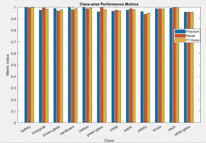
Performance metrics, recalls, and F1 scores by class.
The box plot in Figure 15 shows the performance of the CNN model in accuracy, recall, and waste separation using F1 score metrics. The median accuracy (≈0.99) indicates the model's ability to minimize false positives, whereas the median recall (≈0.98726) emphasizes its ability to detect most positive samples with minimal false negatives despite a slight drop from minimum to minimum range (0.93846) to minimum (0.93846). The F1 score consistently balances accuracy and recall to ensure the robustness of the model. The narrow range and lack of outliers across all metrics demonstrate the stability and reliability of the model across a variety of waste categories, making it suitable for efficient and accurate automated waste management.

Boxplots of accuracy, recalls, F1 scores.
Each data point on the chart corresponds to a specific waste type, such as “trash”, “shoes”, and “plastic”, and can be plotted against the X-axis to represent a sequence of input images. The Y-axis classifies the types of waste detected. CNN successfully identified certain categories such as “green grass” at X = 78, “biology” at X = 224, “shoes” at X = 606, “plastics” at X = 863, and “garbage” at X = 1386. However, categories such as “clothing” and “metals” show variation and potential challenges. This variability can result from overlapping visual features between categories and limitations of model training data. The stepped patterns observed in the plot suggest a sequential classification approach in which the model processes and classifies the inputs one by one. The results highlight the need for further optimization, such as expanding the dataset, using advanced data augmentation techniques, fine-tuning the architecture of the model, and improving detection accuracy for all waste categories, while highlighting the CNN's ability to isolate waste materials. This study demonstrates the applicability of CNNs for automated waste management. This is an important step towards efficient and sustainable recycling practices.

Test prediction graph.
The measured accuracy for training and verification is shown in Figure 16. The blue line represents the accuracy of the training, while the orange line indicates the training loss of the training dataset. The X-axis represents the number of iterations used in the training dataset, while the Y-axis reflects accuracy.
Training and Validation Accuracy Graphs Figure 17 provides insight into the performance of the ResNet model during the learning process. Initially, the training accuracy (blue line) increases sharply as the model learns to classify waste categories. Approximately 100 iterations will stabilize the accuracy and gradually approach close to 100%. The black dotted line indicates that the accuracy of the validation follows a similar trend, reaching a final value of 95.54%, indicating a strong generalization of invisible data. The close alignment between training and validation accuracy across iterations indicates that the model effectively avoids excessive avoiding fitting while maintaining consistency.
Corresponding loss graph Figure 18 provides further evidence of model performance by tracking error reduction on iterations. The orange line represents a loss of training, initially decreasing sharply and indicating rapid learning. Similarly, the black dotted line representing the validation loss follows the same trend and stabilizes at a lower value. The proximity of these lines ensures the robustness of the model, as it successfully minimizes errors in both the training and validation datasets. These graphs show that the ResNet model balances learning efficiency and accuracy.

Training and verification accuracy graphs.

Training and Validation Loss Graph.
Comparisons of predicted and actual labels for 16 randomly selected test samples are visualized in Figure 19. The model is labelled 15 out of 16 objects, showing close match and robust performance. Close to full predictions indicates that ResNet systems can reliably distinguish between different types of decomposeable waste under actual conditions.

The proposed CNN model was trained using an 80:20 training validation split with Adam Optimiser, categorical cross entropy loss, and a batch size of 32 of 150 epochs. Performance was stable after about 100 epochs, accuracy was improved, reduced verification losses were reduced, and learning robustness was demonstrated. Hyperparameter tuning improved model generalization by fine-tuning learning rate (0.0005), dropout (0.2-0.5), and batch size. Data augmentation (inversion, rotation, contrast normalization) was effective in simulating variation in real-world situations and increasing robustness to distortion and occlusion. These improvements culminated with a final classification accuracy of 98.16%. Accuracy and loss plots, and confusion matrix analysis, supported the reduction of misclassification, including differences in visual similarity classes such as green vs white class glass.


