

For a long time I mixed all of this up. Exactly one thing was clear in my head: there’s SFT, where you train the model to predict token after token. After that it turned into soup. RLHF, PPO, DPO, RLVR, GRPO, reward model, value function. A pile of three- and four-letter acronyms all orbiting “fine-tuning”, and it was never clear which one was a cousin of which, and which was from a different universe entirely.
I’m an ML Engineer. My job isn’t to “explain how someone else’s paper works”, it’s to design an architecture for a task, train it, ship it to production, and measure whether the business metric actually moved. From that seat, what I was missing was one simple map: what comes after what, what here is supervised and what is real RL, and why a reward model has nothing to do with RL.
This article is that map. By the end you’ll have what I was missing: what post-training is made of, where the line runs between “we trained a reward model” and “we spun the policy with RL”, and how DPO differs from RLHF in plain terms rather than by a symbol in a formula.
The big picture: post-training is not a single button
First, notation. Let x be the prompt and y the completion (what the model generated in response). Almost everything below is a function of the pair (x, y).
How it actually goes:
1. Pretraining. Teach the model language and the general skill of continuing text. It’s not an assistant yet, just a giant autocomplete.
2. SFT (a.k.a. IFT, instruction tuning). Teach it not to keep continuing the sentence but to answer in a question-answer format. This is the foundation, nothing downstream works without it.
3. Preference alignment (RLHF). We want the model to understand what people like and dislike. We collect preferences (roughly, likes and dislikes on pairs of answers), train a reward model, and spin the policy with RL.
4. RLVR.We want the model strong where the answer is easy to check automatically: math, code. Here the reward comes from a checker, not a trained model.
And off to the side sitsDPO. It’s not “the fifth stage after RLVR”, it’s an alternative way to do step 3. Same preference-alignment goal, but without a separate reward model and without RL. We’ll get to why that’s possible below.
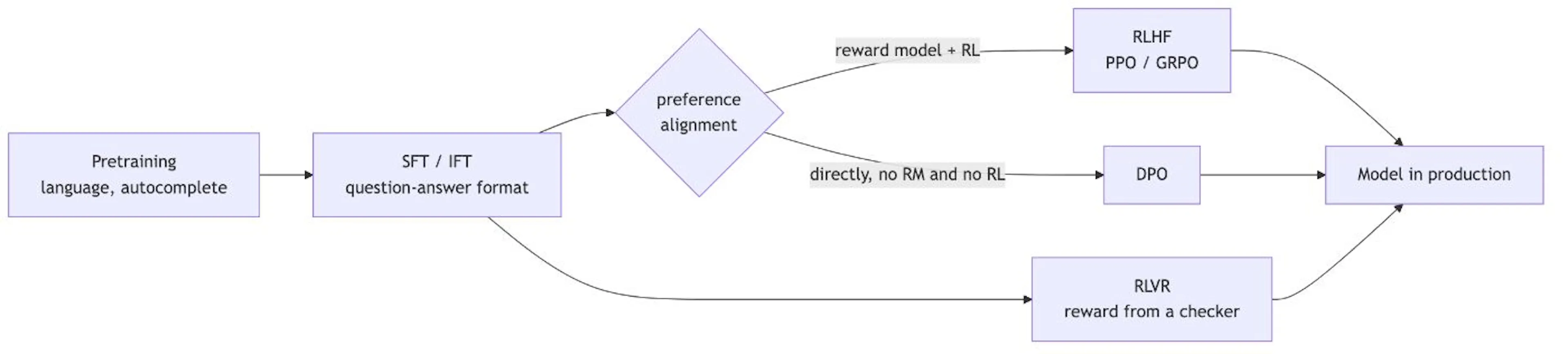 Post-training map
SFT: the same loss as pretraining, but with a mask
A base model after pretraining can do exactly one thing: continue text. Ask it “What is the capital of France?” and it might happily produce “What is the capital of Germany? What is the capital of Italy?”. It isn’t answering, it’s completing a pattern.
SFT fixes exactly this. We show the model data strictly in instruction-answer format and teach it to answer. Technically the loss is the same as in pretraining: autoregressive next-token prediction, plain cross-entropy over the vocabulary. There’s no magic in the loss.
 SFT loss
The whole trick isn’t in the formula, it’s in masking. The prompt tokens x are dropped from the loss, the gradient is computed only over the assistant’s answer y. We don’t want the model learning to predict the user’s questions, we want it learning to answer.
 SFT masking
Reward model: there’s no RL here at all
This is where I got most confused, so let me say it in bold: training a reward model is a supervised task. No policy, no rollouts, no PPO. We’re just training a model that can score answers. The fact that it will later hand rewards to RL doesn’t make its own training reinforcement learning.
Bradley-Terry reward model (from preferences)
The basic variant. We take a pair (prompt x, answer y) and want a single scalar of quality. We stick a small linear head on top of the language model, take the hidden state of the last real token (EOS), and push it through that head. It squeezes the vector into one scalar. We train it with a contrastive loss on pairs: there’s a chosen answer (y_c) and a rejected one (y_r), and the model must give chosen a higher score. Where the loss comes from. The Bradley-Terry model says the probability of preferring i over j is the sigmoid of the difference of their scores:
 Bradley-Terry probability
Hence the negative log-likelihood of the preference:
 Bradley-Terry loss
The important property: only the difference of scores matters. Add a constant to all rewards and the probability doesn’t change. The absolute level of reward is undefined, only the relative one. By the way, this loss is essentially binary cross-entropy: the model predicts a binary “is chosen better than rejected or not”.
The loss itself is trivial. The real difficulty of reward models (like most of post-training) isn’t the math, it’s correct dataloaders and distributed training. They’re usually trained for one epoch to avoid overfitting.
ORM (Outcome Reward Model)
For verifiable domains like math. Same head, different loss: per-token binary cross-entropy on the correctness of the final answer. The label (1 = correct, 0 = incorrect) is copied onto every token of the answer, the prompt is masked. At each token the model predicts the probability that the final answer will be correct. Important caveat: an ORM judges by the final answer only, it won’t catch a mistake in the middle of the reasoning.
PRM (Process Reward Model)
A step up from ORM. We score not just the final answer but every reasoning step. The reasoning is split into steps (usually by newline), and the loss is computed at step boundaries, often as three classes: correct step (+1), neutral (0), wrong (−1). A dense signal instead of a sparse “right or wrong only at the very end”.
Value function
A different beast that lives inside RL (in PPO). The head architecture is like ORM’s (a per-token scalar), but it’s trained on-policy: it estimates the expected remaining reward from the current state and changes together with the policy. It’s a trainable baseline for the advantage, we’ll get to it in the PPO section.
All four in one table:
|
Type |
What it predicts |
How it’s trained |
Head |
|---|---|---|---|
|
RM (Bradley-Terry) |
scalar quality of the whole answer |
contrastive over pairs |
linear on EOS |
|
ORM |
per-token probability of correctness |
BCE, label = outcome |
per-token |
|
PRM |
scores of intermediate steps |
per-step, labels at boundaries |
per-token, 3 classes |
|
Value function |
expected remaining return |
regression, on-policy |
per-token |
A subtlety many trip on: if you train Bradley-Terry on correct/incorrect pairs (chosen = correct answer, rejected = wrong), that’s still a BT model, not an ORM. An ORM is per-token BCE, not contrastive. Different losses, don’t confuse them.
 Reward model heads
Policy gradient: here, finally, is the RL
The overall loop: the policy generates answers, the reward model scores them, the RL optimizer takes a gradient step. And so on for thousands of batches. These are policy-gradient methods, they’re on-policy, meaning they learn from freshly sampled generations, not from an old buffer.
What we’re actually maximizing in RLHF:
 RLHF objective
In plain terms: pull the reward up, but penalize the model for drifting far from the original (reference). `β` is the leash strength, our “KL budget”. Without it, RL as a very strong optimizer will quickly break the model by squeezing everything out of the reward model, artifacts included.
One formula that every algorithm below grows out of:
 Policy gradient
∇log π is the direction to nudge the weights so a token becomes more likely. Ψ_tis a scalar for “how good was this”. Good, push the probability up, bad, push it down. The whole difference between the algorithms comes down to two questions: how to compute `Ψ` (usually the advantage) and how to bound the step size so training doesn’t blow up.
In RLHF, by the way, the discountγ = 1 (no discounting), because the unit of optimization is the whole answer, not a single token.
REINFORCE
The base. We compute the advantage the most naive way: run the batch through the reward model, get a reward per answer, take the batch-mean reward as a baseline, and subtract it from each reward. Then move the gradients.
 REINFORCE loss
The baseline doesn’t bias the gradient but reduces variance. Without it, policy gradient is wildly noisy, especially on sparse rewards.
RLOO (REINFORCE Leave-One-Out)
Almost the same, with one smart trick. When computing the baseline for a given answer, we exclude that answer itself: the baseline is the mean reward of the other answers in the group. Excluding itself makes the estimate unbiased.
 RLOO advantage
No critic, so every token of the answer gets the same sequence-level advantage. You need several answers per prompt.
PPO
This is where it gets harder, and a fourth model appears. PPO uses a value function (critic), a separate trainable model that scores the value of each token. That gives per-token credit assignment (unlike RLOO, where the advantage is one per answer). Canonically the advantage is computed via GAE.
The second key piece is the importance sampling ratio and clipping:
 PPO: importance ratio
Why the ratio: it lets you reuse data collected by the old policy for several gradient steps. And clipping keeps the policy from changing too abruptly in one step. That’s the trust region: keep the step inside a trusted area so it doesn’t blow up. PPO has two losses: a policy loss and a value loss (the critic learns via MSE to the returns).
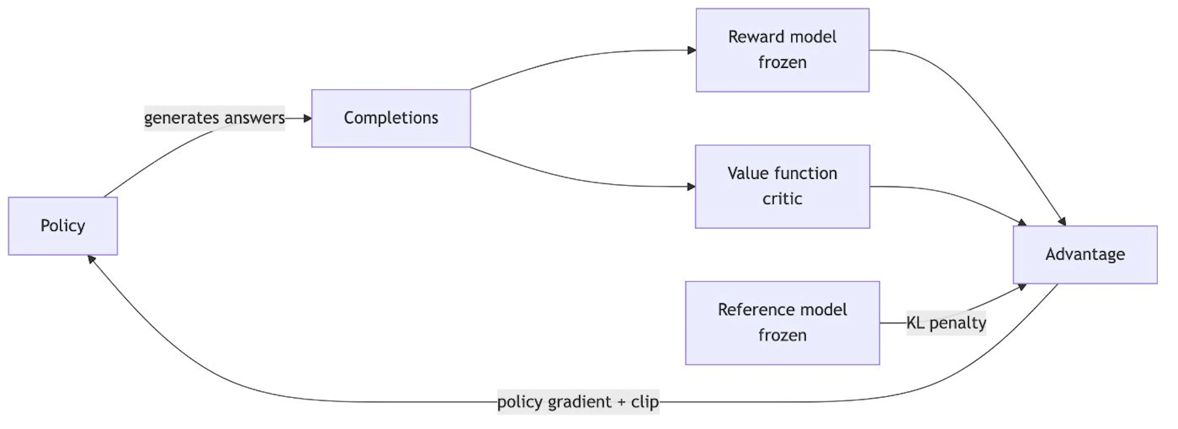 PPO loop with four models
GRPO
Let’s throw out the expensive critic. GRPO is a PPO-like algorithm without a value function. It saves memory: only the policy and the reference are in play.
How we compute the advantage without a critic: generateG answers for one prompt and normalize the rewards within the group, subtracting the mean and dividing by the standard deviation.
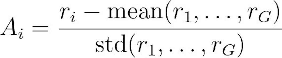 GRPO advantage
Another important implementation difference: GRPO puts the KL penalty straight into the loss (β·D_KL), not into the reward like PPO. The intuition is simple: we compare several answers to one question, pull toward the ones better than their neighbors, and push away from the worse ones.
GSPO and CISPO (fixing instability on long answers and MoE)
These two often get forgotten, but they share one idea: the per-token importance sampling ratio is unstable on long answers and large MoE models. A single token can dominate, or a bunch of tokens get clipped and the signal falls apart.
GSPO (Group Sequence Policy Optimization) is GRPO but with the importance ratio at the whole-sequence level (a length-normalized geometric mean) instead of the token level:
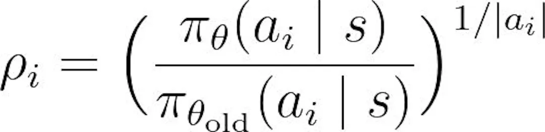 GSPO ratio
The principle: the granularity of the correction should match the granularity of the reward. The reward is over the whole answer, so the correction is too.
CISPO (Clipped Importance Sampling Policy Optimization) comes from the other side: it clips the importance weights themselves, not the objective, and via stop-gradient keeps a gradient on all tokens (REINFORCE-style). It doesn’t throw away the gradients of rare but important tokens.
A summary of the whole ladder:
|
Algorithm |
How it computes the advantage |
Critic |
Where KL goes |
Granularity |
|---|---|---|---|---|
|
REINFORCE |
return − baseline |
no |
in the reward |
answer |
|
RLOO |
leave-one-out over the group |
no |
in the reward |
answer |
|
PPO |
GAE via the value function |
yes |
in the reward |
in the reward (per-token) |
|
GRPO |
group-relative (mean/std) |
no |
in the loss |
answer |
|
GSPO |
like GRPO, but seq-level ratio |
no |
in the loss |
answer |
|
CISPO |
clips weights, all tokens keep a gradient |
no |
in the loss |
token, nothing dropped |
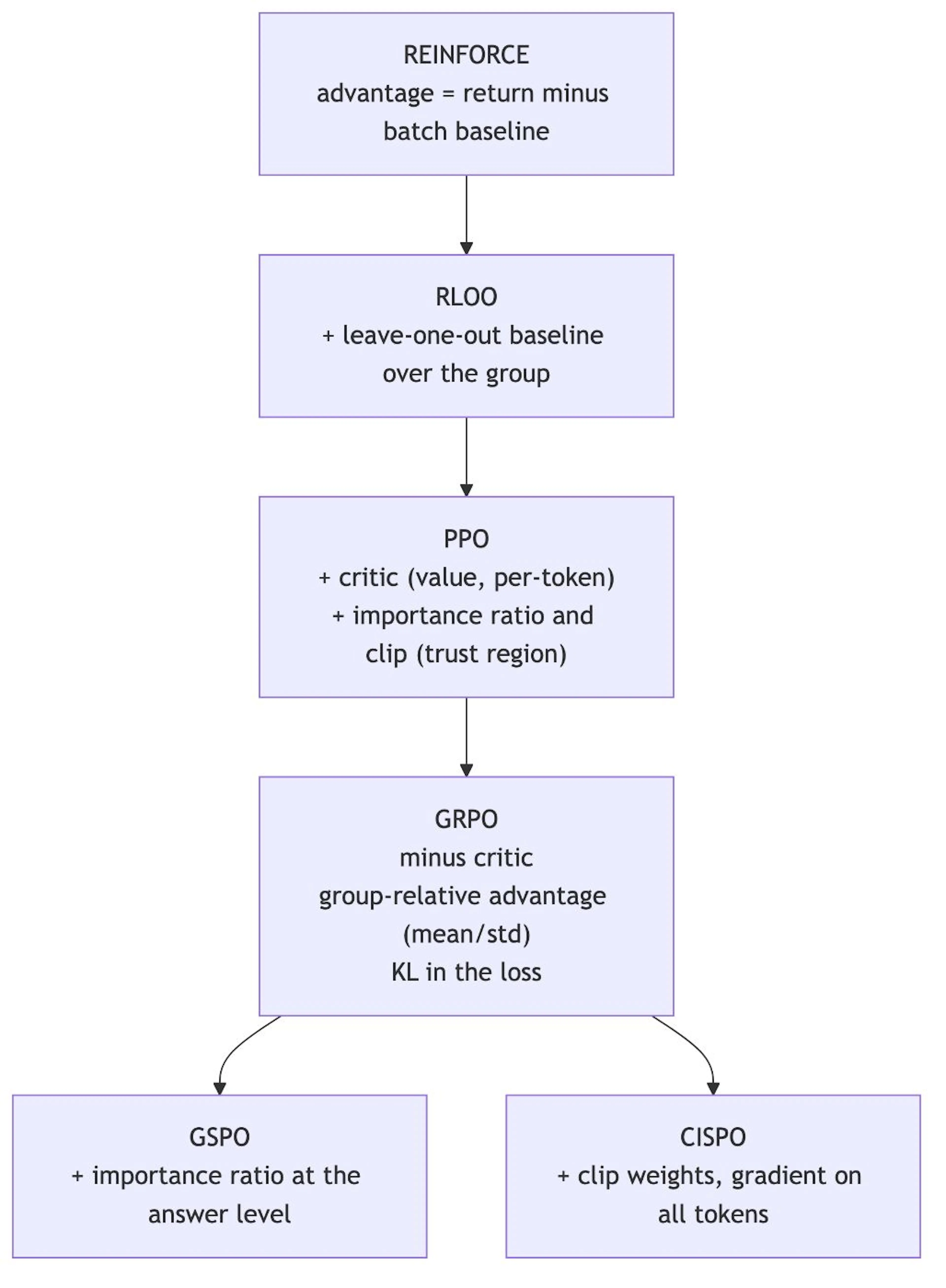 The algorithm ladder
DPO: alignment without a reward model and without RL
Now the fork itself. DPO solves the same alignment problem, but without training a separate reward model and without an RL loop. On the same data: chosen/rejected preference pairs.
The trick: we don’t train a separate reward model. Instead the reward is baked straight into the policy through the log-ratio to the reference:
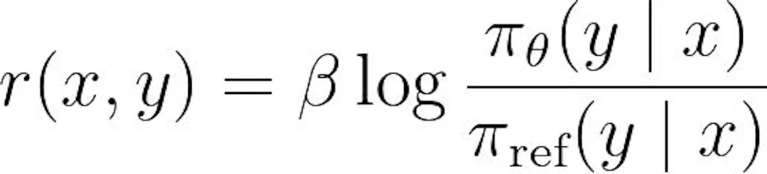 DPO implicit reward
Hence the famous “your language model is secretly a reward model”. Plug that into the same Bradley-Terry and you get a direct contrastive loss on pairs:
 DPO loss
DPO widens the gap between the log-probabilities of chosen and rejected. From the user we know the preference label (that chosen is better), while the reward scalar stays implicit, we never compute it. In the derivation the intractable partition function cancels out, and that’s the beauty of the trick.
In practice DPO fits into a normal training stack, you just need one more reference model for a forward pass (its log-probs can be computed once and cached). The KL here is static, set by `β`, it doesn’t float like in RL.
In production I almost always reach for DPO first rather than standing up a full RLHF loop. Not because DPO is “better” (online RL beats it, if only by a hair), but because data matters more than the algorithm, and DPO lets you iterate far faster and cheaper. A full PPO loop with four models is a separate piece of infrastructure, worth deploying once you’ve hit the ceiling of the offline approach. With reasoning models the pendulum has swung back toward RL, but as a first step DPO almost always wins on effort-to-result.
RLVR: when you don’t have to guess the reward
RLVR (Reinforcement Learning with Verifiable Rewards) is RL where the answer can be checked automatically. Math (did the numeric answer come out right), code (did the tests pass). No trained reward model is needed here, a deterministic checker plays its role: correct, reward 1, wrong, reward 0.
Algorithmically it’s the same policy gradient (most often GRPO), just with a different reward source. A verifier instead of a reward model. And by the way, in the RLVR era the KL penalty is often turned off entirely, to let the model wander further toward strong reasoning.
Putting the map back together
If I squeeze it all into a few lines I wish I’d read at the very start:
- SFT: supervised, the same next-token loss as pretraining but with the prompt masked. Teaches format.
- Reward model: also supervised, no RL. A contrastive loss on pairs (Bradley-Terry), a scalar off the EOS. ORM and PRM for verifiable domains.
- Policy gradient (RLHF): here’s the actual RL. All the algorithms are one formula, differing only in how they compute the advantage and how they keep the step stable.
- DPO: a bypass of RLHF without a reward model or RL, with an implicit reward. Simpler and faster, but offline.
- RLVR: RL where the reward comes from a checker, not a trained model.
The line I now always keep in my head:a reward model is not RL. Training a reward model and optimizing a policy with RL are two different stages with different losses, and they shouldn’t be confused.


