A1. Support vector machine
The Support Vector Machine is. a machine learning model divided into two parts — support vector regression (SVR) and support vector classification (SVC), which can be used for regression and classification76. Regression aims to find a model that can explain the output based on the given input. One of the main advantages of the support vector regression model is that its computational complexity does not depend on the dimensions of the input space. Suppose that the regression function is as Eq. A125.
$$\:f\left(x\right)=\langle{w,x}\rangle+b\:\:\:\:\:\:\:\:\:\:\:\:\:\:\:\:\:\:\:\:\:\:\:\:\:\:\:\:\:with\:w\in\:X\:,\:b\in\:\mathbb{R}$$
(A1)
The main purpose. is determining the optimal separating hyperplane that can be achieved by solving the following convex quadratic problem (Eq. A2)77.
$$\begin{aligned}\:\phi\:\left(w,\xi\:\right)=\frac{1}{2}{\parallel{w}\parallel}^{2}+C\sum\:_{i=1}^{\mathcal{l}}\left({\xi\:}_{i}+{\xi\:}_{i}^{\text{*}}\right)\\\:subject\:to\:\left\{\begin{array}{c}{y}_{i}-\left(\langle{w},{x}_{i}\rangle+b\right)\le\:\epsilon\:+{\xi\:}_{i}\\\:\left(\langle{w},{x}_{i}\langle+b\right)-{y}_{i}\le\:\epsilon\:+{\xi\:}_{i}^{\text{*}}\\\:{\xi\:}_{i},{\xi\:}_{i}^{\text{*}}\ge\:0\:\:\:\:\:\:\end{array}\right.\end{aligned}$$
(A2)
where \(\:{x}_{i}\) is an input datum. \(\:<.,.>\) denotes the inner product, \(\:w\) is the normal vector of the hyperplane, and \(\:b\) is a scalar value considered the bias parameter. The constant \(\:C\) is the penalty factor and is selected by the user. The value of \(\:\epsilon\:\) defines a margin of tolerance where no penalty is given to errors; for any value that falls outside of \(\:\epsilon\:\), we can denote its deviation from the margin as \(\:\xi\:\). Refer to Smola and Schölkopf 25 for more details about SVR.
The performance of the SVR model. depends on its learning parameters, such as the maximum deviation from targets (\(\:\epsilon\:\)), penalty factor (\(\:C\)) and kernel deviation (\(\:\sigma\:\)). \(\:\sigma\:\) is effective in converting input data into feature space and controls the complexity of the model. However, finding the best combination of these hyperparameters is difficult due to the nonlinear nature of the model. This study aims to find its optimal values.
A2. Convolutional neural network
Convolutional Neural Network (CNN). is a deep learning model that can extract spatial patterns from input data using convolutional filters10,24,26. Unlike ordinary neural networks, CNN can preserve the local structure of input data and use neighboring pixels in the learning process. Therefore, CNN has been used in different spatial prediction and susceptibility mapping studies, especially when the spatial arrangement of the conditioning factors is important[10,24,26].

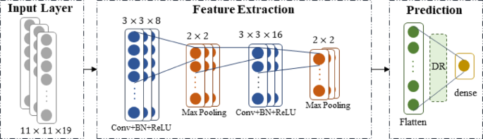
CNN architecture used in this study, adapted from Jafari et al.10
In this study, the CNN architecture was adopted from Jafari. et al.10 and is shown in Figure A1. This architecture includes convolutional blocks for feature extraction and fully connected layers for final prediction. In the convolutional part, the input data are processed using convolutional filters, followed by batch normalization, ReLU activation function, and max pooling layers. These layers extract spatial features and reduce the dimension of the feature maps. After feature extraction, the flatten layer converts the extracted feature maps into a one-dimensional vector. Then, the dropout layer is applied to reduce overfitting, and the fully connected layer is used to generate the final prediction78.
The performance of CNN depends on both the selected input features and the hyperparameter values used during the training process10,26. Therefore, in this study, the CNN hyperparameters were optimized simultaneously with feature selection using the proposed TGWO and MSQLTGWO algorithm. The optimized hyperparameters included the initial learning rate, learn rate drop factor, learn rate drop period, mini-batch size, and dropout rate10. The initial learning rate controls the speed of model learning during training. The learn rate drop factor and learn rate drop period control the reduction of the learning rate during the training process. The mini-batch size determines the number of samples used in each training iteration, and the dropout rate controls the proportion of neurons that are temporarily ignored to reduce overfitting78. Therefore, optimizing these hyperparameters can improve the CNN learning process and predictive performance.
A3. Grey wolf optimizer (GWO)
This algorithm was initially presented by Mirjalili et al. 79. The GWO is a population-based and hierarchical algorithm and originated from grey wolves hunting behavior79. The advantages of the GWO algorithm are fast search speed, high search precision, and modeling simplicity. There are four types of grey wolves in this algorithm, namely alpha (\(\:\alpha\:\)), beta (\(\:\beta\:\)), delta (\(\:\delta\:\)), and omega (\(\:\omega\:\)). The alpha wolf is the group leader that decides about sleeping, waking time, hunting. The beta wolf helps the alpha in decision-making. The delta wolves obey alphas and betas. At the last level of the grey wolves is the omega wolf. Omega wolves must always obey alpha, beta, and delta wolves80. The algorithm’s operation includes four phases: encircling prey, hunting, attacking, and searching for prey.
I. Encircling prey.
In its initial stage of hunting, grey wolves surround the prey with a distance of \(\:\overrightarrow{D}\) (Eq. A3-4).
$$\:\overrightarrow{D}=\left|\overrightarrow{C}\bullet\:{\overrightarrow{X}}_{p}\left(t\right)-\overrightarrow{X}\left(t\right)\right|$$
(A3)
$$\:\overrightarrow{X}\left(t+1\right)={\overrightarrow{X}}_{p}\left(t\right)-\overrightarrow{A}\bullet\:\overrightarrow{D}$$
(A4)
where \(\:t\) denotes the current iteration. \(\:\overrightarrow{X}\left(t\right)\) and \(\:{\overrightarrow{X}}_{p}\left(t\right)\) are the position vector of the grey wolves and the prey, respectively. \(\:\overrightarrow{A}\) and \(\:\overrightarrow{C}\) represent the vectors of coefficients. They are estimated by Eqs. A5-6.
$$\:\overrightarrow{A}=2\overrightarrow{a}\bullet\:{\overrightarrow{r}}_{1}-\overrightarrow{a}$$
(A5)
$$\:\overrightarrow{C}=2\bullet\:{\overrightarrow{r}}_{2}$$
(A6)
In which \(\:\overrightarrow{a}\) is linearly reduced from 2 to 0, and \(\:{\overrightarrow{r}}_{1}\),\(\:\:{\overrightarrow{r}}_{2}\) are random vectors between \(\:\left[\text{0,1}\right]\).
II. Hunting.
In this phase, it is assumed that \(\:\alpha\:\), \(\:\beta\:,\) and \(\:\delta\:\) wolves have a good knowledge of prey’s position, so hunting is guided by these three types of grey wolves, respectively. The mathematical model of this behavior is shown as Eqs. A7 and A8.
$$\:{\overrightarrow{\varvec{D}}}_{\varvec{\alpha\:}}=\left|{\overrightarrow{\varvec{C}}}_{1}\bullet\:{\overrightarrow{\varvec{X}}}_{\varvec{\alpha\:}}-\overrightarrow{\varvec{X}}\right|,\:{\overrightarrow{\varvec{D}}}_{\varvec{\beta\:}}=\left|{\overrightarrow{\varvec{C}}}_{2}\bullet\:{\overrightarrow{\varvec{X}}}_{\varvec{\beta\:}}-\overrightarrow{\varvec{X}}\right|,\:{\overrightarrow{\varvec{D}}}_{\varvec{\delta\:}}=\left|{\overrightarrow{\varvec{C}}}_{3}\bullet\:{\overrightarrow{\varvec{X}}}_{\varvec{\delta\:}}-\overrightarrow{\varvec{X}}\right|$$
(A7)
$$\:{\overrightarrow{\varvec{X}}}_{1}={\overrightarrow{\varvec{X}}}_{\varvec{\alpha\:}}-{\overrightarrow{\varvec{A}}}_{1}\bullet\:\left({\overrightarrow{\varvec{D}}}_{\varvec{\alpha\:}}\right),\:{\overrightarrow{\varvec{X}}}_{2}={\overrightarrow{\varvec{X}}}_{\varvec{\beta\:}}-{\overrightarrow{\varvec{A}}}_{2}\bullet\:\left({\overrightarrow{\varvec{D}}}_{\varvec{\beta\:}}\right)\:,\:{\overrightarrow{\varvec{X}}}_{3}={\overrightarrow{\varvec{X}}}_{\varvec{\delta\:}}-{\overrightarrow{\varvec{A}}}_{3}\bullet\:\left({\overrightarrow{\varvec{D}}}_{\varvec{\delta\:}}\right)$$
(A8)
where \(\:{\overrightarrow{X}}_{\alpha\:}\), \(\:{\overrightarrow{X}}_{\beta\:}\), and \(\:{\overrightarrow{X}}_{\delta\:}\) indicate the location of the alpha, beta, and delta wolves, respectively. The updated location of the grey wolf in the search space is calculated by Eq. A9.
$$\:\overrightarrow{\varvec{X}}\left(\varvec{t}+1\right)=\frac{{\overrightarrow{\varvec{X}}}_{1}+\:{\overrightarrow{\varvec{X}}}_{2}+\:{\overrightarrow{\varvec{X}}}_{3}}{3}$$
(A9)
The other wolves update their positions randomly around the prey’s position.
III. Attacking prey (exploitation).
When the prey stops moving, the grey wolf terminates the hunt. It should be noted that \(\:\overrightarrow{A}\) is randomly generated in the interval \(\:\left[-2a\:,\:2a\right]\) and decreases linearly by \(\:a\). The exploitation operation is finished when \(\:\left|A\right|<1\) and \(\:\left|C\right|<1\).
IV. Search for prey (exploration).
Grey wolves search for prey based on the position of \(\:\alpha\:\), \(\:\beta\:,\) and \(\:\delta\:\). Therefore, alpha, beta, and delta grey wolves play a guiding role in this section. The searching of prey process is the opposite of the attacking process. Grey wolves diverge and distribute for searching of the prey when \(\:\left|A\right|>1\). After tracking the prey, they approach each other in the attack phase. The coefficient \(\:\overrightarrow{C}\) is considered as an obstacle in nature that slows down grey wolves approaching prey.
For every iteration, the position of the alpha, beta, and delta wolves are estimated first, and then the locations of the other answers are determined. At the end of the iteration, the alpha wolf position will be introduced as the optimal position.
A4. GWO-augmented strategies
This section details the strategies used to enhance the GWO. By incorporating principles from evolutionary metaheuristic algorithms, these strategies improve the standard GWO.
I. Soft-rime and Hard-rime.
Soft-rime (SR) and Hard-rime (HR) are two strategies utilized in the Rime Optimization Algorithm (RIME)81, which is inspired by the natural phenomenon of rime. The SR strategy is inspired by the growth of soft rime agents in a gentle breeze, which exhibit highly irregular and extensive movement. Consequently, SR explores the entire search space during the initial iterations, preventing the algorithm from getting trapped in local optima. The mathematical model for the SR strategy is represented by Eqs. A10-A13 and Algorithm A1.
$$\:{X}_{ij}^{new}=\:{X}_{best,j}+{r}_{1}\:.\:cos\theta\:\:.\:\gamma\:\:.\:\left(h\:.\:\left(ub-lb\right)+lb\right),\:\:\:\:\:\:{r}_{2}
(A10)
$$\:\theta\:=\:\pi\:\:.\:\frac{It}{10\:.\:MaxIt}$$
(A11)
$$\:\gamma\:=1-\:\frac{\left[\frac{w\:.\:It}{MaxIt}\right]}{w}$$
(A12)
$$\:L=\:\sqrt{\frac{It}{MaxIt}}$$
(A13)
where, \(\:i\) and \(\:j\) denotes \(\:j-th\) particle of the \(\:i-th\) rime-agent, \(\:{X}_{ij}^{new}\) is the new position, \(\:{X}_{best,\:j}\) is \(\:j-th\) particle of the best rime-agents in the population,\(\:{r}_{1}\) is random number in the range (-1, 1), \(\:{r}_{2}\) and \(\:h\) are random number in the range (0, 1), \(\:lb\) and \(\:ub\) are lower band and upper band of rime-agents, and \(\:w\) controls the number of segments of the step function and is set to 5 based on standard RIME81.

Pseudo-code of the soft-rime search strategy[81].
The HR strategy is inspired by the growth of hard-rime particles in a severe storm, which exhibit a simpler and more regular movement compared to the growth of soft-rime particles. Hard particles tend to grow uniformly in one direction, facilitating the rime piercing phenomenon where elements easily intersect. Consequently, the HR strategy aims to increase convergence efficiency and escape local optima through interaction and exchange among the search agents. The mathematical model for the HR strategy is represented by Eq. A14 and Algorithm A2.
$$\:{X}_{ij}^{new}=\:{X}_{best,j},\:\:\:\:\:\:{r}_{3}<{F}^{normr}\left({S}_{i}\right)\:$$
(A14)
where, i and j denotes j-th particle of the i-th rime-agent, Xij new is the new position, Xbestj is j-th particle of the best rime-agents in the population, r3 is random number in the range (-1, 1), and Fnormr value represents the normalized fitness value of the current rime-agent.

Pseudo-code of the hard-rime puncture mechanism [81].
II. Dispersed foraging method.
When a food shortage event occurs in an area with a pack of wolves, the dispersed foraging method forces some wolves to disperse into a new area to search for food82. The mathematical modeling of this concept is carried out in accordance with the Eqs. A15 and A1683 and Algorithm A3. According to these equations, during the food search phase, some wolves can disperse to a new area at a dispersal rate \(\:DR\), which prevents them from being trapped in a local optimum46,82.
$$\:DR=\:{DR}_{max}-\left({DR}_{max}-\:{DR}_{min}\right)\:.\:\frac{It}{MaxIt}$$
(A15)
$$\:X\left(t+1\right)=\:\left\{\begin{array}{c}\begin{array}{cc}X\left(t\right)+\:\rho\:\:.\:\left({X}_{m}\left(t\right)-\:{X}_{n}\left(t\right)\right),\:\:&\:if\:r>DR\end{array}\\\:\begin{array}{cc}X\left(t\right),&\:otherwise\end{array}\end{array}\right.$$
(A16)
where, m and n are random search agents, \(\:\rho\:\) is a scaling factor with distribution \(\:\rho\:\:\sim\:(0.5,\:{0.1}^{2})\), r is random number in the range (0, 1), and based on study83\(\:{DR}_{max}=0.4\) and \(\:{DR}_{min}=0.0\).

Pseudo-code of dispersed foraging process.
A5. Q-learning
Q-learning is one of the most common and important reinforcement learning algorithms84,85. In reinforcement learning, Q-learning is an algorithm for taking appropriate actions \(\:A=\{{a}_{1},\:{a}_{2},\:\dots\:,\:{a}_{n}\}\) in states \(\:S=\{{s}_{1},\:{s}_{2},\:\dots\:,\:{s}_{m}\}\) based on the cumulative reward during the process of agents interacting with the environment. According to Figure A2, an agent performs an action \(\:{a}_{t}\), transitions from state \(\:{s}_{t}\) to \(\:{s}_{t+1}\), and receives a reward \(\:{r}_{t+1}\) based on its interaction with the environment. Then, based on the received reward, \(\:Q({s}_{t},\:{a}_{t})\), which is the cumulative reward value of a state-action pair at time \(\:t\), is updated according to Eq. A17 and stored in the Q-table.
$$\:{Q}_{new}\left({s}_{t},\:{a}_{t}\right)=\:Q\left({s}_{t},\:{a}_{t}\right)+\:\alpha\:\:\times\:[{r}_{t+1}+\:\gamma\:\:{max}_{a}Q\left({s}_{t+1},\:a\right)-\:Q\left({s}_{t},\:{a}_{t}\right)]$$
(A17)
where, \(\:{Q}_{t}\:\)is the expected Q in current state and \(\:{Q}_{t+1}\) is represents the expected value of Q in the next state, \(\:\alpha\:\) and \(\:\gamma\:\) are learning rate, and discount rate. In this study, \(\:\alpha\:=0.1,\:\gamma\:=0.9\) 71.

Diagram of reinforcement learning.
In the action selection phase of the Q-learning algorithm, there are two approaches. The first approach is for the agent to select a completely random action to discover unknown paths (exploration). Alternatively, it can select the action that has the highest value in the Q-table for the current state. This allows the agent to utilize the knowledge it has previously acquired (exploitation). Finally, the cycle shown in Figure A2 is repeated multiple times until the Q-table values stabilize and specify the optimal action for each state that yields the maximum reward.

Pseudo-code of the Q-learning algorithm[86].