

We present our results in the upcoming sections by following these steps. First, we trained five base classifiers for each data representation. Then, we performed cross-validation to determine the best classifier for each representation. Next, we combined the data representations into ensemble classifiers using a two-stage ensemble selection strategy. The first stage prunes candidates for an ensemble classifier. The second stage searches for the optimal subset of the remaining candidates. Third, we evaluated the best ensemble classifier and compared it with the best base classifier. Finally, we assessed the performance of the best ensemble classifier on the GI boundaries prediction task. We conducted our study using the Benbow dataset.
Performance of different data representations and classifiers
To understand the performance of different data representations and classifiers, we cross-validated diverse combinations of data representations and classifiers (see Methods for more details). We performed a 5-fold StratifiedGroupKFold cross-validation, which we repeated 5 times, and reported the average Matthew correlation coefficient (MCC) for each combination of data representation and classifier. Stratification was done at the species level to ensure distinct sets of species in the training and validation datasets.
Figure 1a shows a heatmap of the cross-validation results, which corresponds to Fig. 1a from our previous study9. We found that random forest (RF) is more robust to data representation than other classifiers. However, SVM outperforms RF in certain data representations. For k-mer-based representations, RF performance declines from k-mer 4 to k-mer 7, while SVM performance increases as the k-mer size increases. This suggests that SVM is more robust for longer data representations than RF. To avoid using the same data representation, we selected the best-performing classifier for each representation, as shown in Fig. 1b. Ultimately, there are 44 candidates, which is equivalent to the number of data representations.
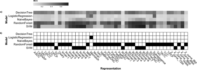
(a) Cross-validation results for various model and representation combinations. The color coding represents the Matthew correlation coefficient (MCC). The darker the color, the higher the value. (b) The selected model for each data representation is shown. Black boxes represent the selected classifier for each data representation. The x-axis displays the data representations and the y-axis depicts the base classifiers.
Ensemble classifiers
A two-stage ensemble selection strategy was implemented to construct ensemble classifiers. First, the pool of candidates for the ensemble classifier was reduced to narrow the search. Second, an ensemble growth strategy was used to select the optimal subset of candidates.
The pruning process was formulated as a multi-objective optimization problem with two objectives: maximizing diversity and minimizing the error rate. Diversity was measured using Cohen’s kappa agreement21, while the error rate was quantified by \(1-MCC\). Two pruning solutions, Pareto frontier (pfront) and convex hull (chull), were applied by following a study on encoding selection with ensemble pruning15.
Figure 2 shows an example of a kappa-error diagram, where the x-axis represents the kappa agreement between pairs of candidates and the y-axis shows the average error rate between them. We provided the kappa-error diagrams of all cross-validation folds in Supplementary Fig. S1 for visual comparison only.

Example of a Kappa-error diagram from one fold in cross-validation. Each dot represents a pair of candidates (one data representation and one classifier). The gray dots correspond to all possible pairs of candidates. The green dots represent pairs selected by the convex hull, and the purple dots represent pairs selected by the Pareto frontier. The optimal solution for the ensemble classifier should have a low average error rate and low Kappa, indicating high diversity, and is located in the lower left part of the diagram. The error rate is defined as \(1-MCC\), where MCC is Matthew correlation coefficient. An average error rate is the average error rate of each candidate in a pair.
Since there were potentially many candidates, we limited the number to 20. In addition to the pfront and chull solutions, Spänig et al.15 selected the 15 best-performing encodings. We selected the top 20 candidates as the optimal subset solely based on their performance (MCC) in the cross-validation results; thus, we used 3 solutions to select the candidates: pfront, chull, and best. After narrowing down the candidates, we used an ensemble growing procedure to select the optimal subset for the ensemble classifier. We applied 3 ensemble methods: voting_soft, voting_hard, and stacking.
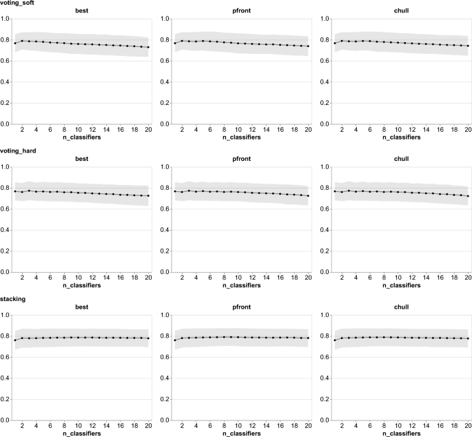
Ensemble learning performance is evaluated with different numbers of base classifiers across different ensemble methods and solutions. voting_soft, voting_hard, and stacking ensemble methods were used. For the ensemble solutions, we used Pareto frontiers (pfront), convex hulls (chull), and the best base classifiers to select candidates for ensemble learning. The solid line shows the mean Matthew correlation coefficient (MCC), and the shaded band represents the standard deviation across cross-validation folds. Five-fold cross-validation was repeated five times.
Figure 3 illustrates the cross-validation results for ensemble classifiers that have different numbers of base classifiers. On the one hand, we observed a similar trend in ensemble classifiers with voting strategies, wherein the performance increased when the number of base classifiers was increased up to a certain value (2 and 3 for voting_soft and voting_hard, respectively), and subsequently decreased as the number of base classifiers grew. On the other hand, the performance of ensemble classifiers with stacking exhibited relative stability irrespective of the size of the ensemble classifier. This phenomenon can be attributed to the use of a meta learner in the stacking method. A meta learner can combine the predictions of multiple base classifiers. Ensemble classifiers with voting, on the other hand, depend on the performance of base classifiers.
Table 1 shows the selected candidates for each ensemble method and solution that yields the best ensemble model. We observed that RCKmer-7 with SVM and subsequence with random forest were selected in all methods and solutions. RCKmer-7 with SVM was selected because it performed the best individually, whereas subsequence with random forest did not perform as well as RCKmer-7 with SVM. Among other candidates with similar performance, subsequence with random forest was selected because it offered higher diversity. Thus, when both candidates were combined in an ensemble classifier, they performed better than they did individually.
In comparison to voting strategies, the stacking method achieved the best performance with relatively more classifiers. Although adding more classifiers in ensemble learning with stacking gives an improvement, the gain is not as much as adding one classifier to the best base classifier; thus, similar performance can be achieved with fewer classifiers. Furthermore, we conducted a statistical test, namely the corrected repeated k-fold cv test22, to compare the performance of the best base classifier and the ensemble classifiers. The statistical test indicated that there is no significant difference between the base best classifier and all ensemble classifiers, except the voting_soft ensemble (\(p=0.033\)). After applying the Bonferroni-Holm correction, we found no ensemble classifier statistically outperforming the single classifier.

Difference performance between single and ensemble classifiers across cross-validation folds for all ensemble methods and solutions. Differences were calculated on the same fold.
Additionally, we analyzed the performance differences measured by MCC between single and ensemble classifiers across all cross-validation folds, as depicted in Fig. 4. The stacking ensemble demonstrated the highest variance in performance differences, while the voting_hard ensemble showed the least variance. The voting_soft ensemble exhibited intermediate variance but achieved the highest average performance differences compared to the single classifier. Consequently, the voting_soft ensemble (comprising RCKmer-7/SVM and Subsequence/RF) was chosen as the ensemble classifier for further analysis in this study, where it was compared to the best single classifier (RCKmer-7/SVM).
Heterogeneous vs homogeneous base classifiers
Our approach to ensemble selection differs from Spänig et al.15, which combines different data representations with the same base classifier. Here, we investigated whether combining data representations with heterogeneous base classifiers is better than with homogeneous base classifiers. We performed the two-stage ensemble selection strategy on 5 base classifiers and compared the results with our study.
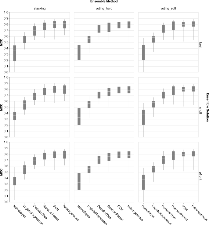
A comparison of Matthew correlation coefficient (MCC) between ensemble classifiers with two different base classifiers types: heterogeneous and homogeneous. Each row represents the ensemble solutions (pareto frontier, convex hull, and best), and each column displays the ensemble methods (stacking, voting_hard, voting_soft). Heterogeneous base classifiers significantly outperformed homogeneous base classifiers across all ensemble methods and solutions (corrected repeated k-fold cv test22 \(p<0.05\)), except decision tree, random forest, and SVM.
The boxplot in Fig. 5 shows a comparison of ensemble and homogeneous base classifiers. Across all ensemble methods and solutions, heterogeneous base classifiers demonstrated higher performance levels than homogeneous base classifiers. However, corrected repeated k-fold cv tests22 with Bonferroni-Holm correction indicated that heterogeneous base classifiers significantly outperformed homogeneous base classifiers across all ensemble methods and solutions, except Decision Tree, Random Forest, and SVM (\(p>0.05\)).
Evaluate ensemble classifier
After finding the best ensemble classifier, we compared it with the best single classifier on two tasks, which are classification and GI boundaries prediction task. We trained both classifiers on the entire Benbow training dataset and evaluated them using the Benbow test dataset, which consists of 20 genomes. Then, we used the same trained classifiers on the GI boundaries prediction task. Additionally, we reported the performance of another candidate in the ensemble classifier, which is Subsequence/Random Forest.
Initially, we selected the voting_soft ensemble method, but it performed sub-optimally in the boundary prediction task compared to the single classifier, despite outperforming it in the classification task. As an alternative, we also evaluated the stacking ensemble method. We compared the performance of the single classifier, ensemble classifier with voting_soft, and stacking on the entire Benbow test dataset.
Evaluation on classification task

Comparison of the best single classifier (RCKmer-7/SVM), Subsequence/Random Forest, ensemble classifier with voting_soft, and stacking on the Benbow test dataset. (a) Confusion matrices showed both ensemble classifiers captured more positives than the single classifier. 0 is the negative class and 1 is the positive class. (b) The left figure shows the Matthew correlation coefficient (MCC) of each classifier across 20 species, whereas the right figure shows the number of positive and negative samples per species. The ensemble classifiers are better than the single classifier on some species, but they were outperformed by single classifiers on 6 species (NC_009665.1, NC_009512.1, NC_010334.1, NC_009504.1, NC_007432.1, and NC_004070.1).
Figure 6a shows confusion matrices of all classifiers. Both ensemble classifiers were more effective in capturing positive instances compared to the single classifier, with the stacking ensemble method identifying even more positives than the voting_soft method. Furthermore, we analyzed their performance across 20 species in the test dataset. The left bar chart in Fig. 6b shows the MCC comparison of all classifiers across 20 species, whereas the right bar chart displays the number of positives and negatives per species. The ensemble classifiers were overall superior to the single classifiers, but they were outperformed by either the single classifier or Subsequence/Random Forest on 6 species (NC_009665.1, NC_009512.1, NC_010334.1, NC_009504.1, NC_007432.1, and NC_004070.1). NC_009665.1 and NC_010334.1 are representatives of the genus Shewanella, identified as Shewanella baltica OS185 and Shewanella halifaxensis HAW-EB4; NC_009512.1 corresponds to Pseudomonas putida F1; NC_009504.1 is Shewanella halifaxensis ATCC 25840 chromosome II; NC_007432.1 and NC_004070.1 belong to genus Streptococcus (Streptococcus agalactiae A909 and Streptococcus pyogenes MGAS315, respectively). Replacing voting_soft with stacking showed both improvement and a drop in performance on certain species. None of the ensemble classifiers could successfully distinguish positive from negative classes for NC_004070.1 (Streptococcus pyogenes MGAS315), which had the fewest samples.
Overall, the ensemble classifiers (Recall: 0.966 and 0.978 for voting_soft and stacking, respectively) achieved higher recall than the single classifier (Recall: 0.959), highlighting its ability to capture positive classes better. However, it is noteworthy that there is a different positive class ratio between training and test datasets. The test set contains 566 sequences from 20 genomes, with 413 positives (73.0% positive) compared to 1,329 positives out of 2,569 sequences (51.7% positive) in the training of 147 genomes. This 21.3% point shift toward higher positive prevalence may influence Recall estimates, as models trained on more balanced data can appear to have higher Recall when evaluated on a positive-enriched dataset. To address this, we provided bootstrapped confidence intervals on all evaluation metrics in Table 2, where the ensemble consistently outperforms the single classifier in Recall (0.979 vs 0.959), F1 score (0.962 vs 0.953), MCC (0.854 vs 0.824), and Accuracy (0.944 vs 0.931), except Precision (0.946 vs 0.947), all with 95% bootstrap confidence intervals. These increases in prevalence-robust metrics suggest that the benefits of the ensemble method surpass the effects of distribution shifts that favor the Recall. However, McNemar’s exact test on per-sample paired predictions (n=566 samples) indicated no significant difference between single and ensemble classifiers (\(p=0.18\) and \(p=0.07\) for voting_soft and stacking, respectively). Notably, the ensemble classifier identified 9 samples that were missed by the single classifier, while there were 6 and 2 samples (voting_soft and stacking, respectively) with errors that were unique to the ensemble. This improvement might seem negligible, but this is highly important for the GIs detection.
Evaluation on boundaries prediction task
To test the performance of the ensemble classifier to localize GIs, we adopted an existing pipeline for predicting GI boundaries developed by Banerjee et al.24 and replaced the ML model with the ensemble and single classifiers. The existing pipeline uses a sliding window approach to scan a genome and predict GI boundaries. The pipeline determines the confidence of its classification of a window as a GI segment depending on the probability of that window. To assign a class to each window, it applies a lower and upper threshold. The lower threshold is set to 0.5 and the upper threshold is set to 0.8. If the probability of a given window falls below the lower threshold, the window is labeled as the negative class and it is not processed further. Otherwise, if the probability exceeds this upper threshold, the pipeline can classify it as the positive class. Any windows with probabilities between the lower and upper thresholds will undergo further processing of a boundary refinement step (see Fig. 3 in24). To ensure a fair comparison, we used the default hyperparameters of the pipeline with a window size of 10,000 base pairs (bp), a lower threshold of 0.5, and an upper threshold of 0.8.
In addition to the comparison between the best ensemble and single classifiers, we provided a comparison with other baselines that were reported in our previous study9. Predictions of other baselines are available in https://github.com/FriedbergLab/GenomicIslandPrediction/tree/master/evaluation/predictions24. We additionally trained the single classifier (RCKmer-7/SVM) with the best hyperparameters found in our previous study (kernel: ’rbf’, C: 2, gamma: ’scale’). To make a fair comparison, we also trained both ensemble classifiers (voting_soft and stacking) with the best hyperparameter for RCKmer-7/SVM, but used default hyperparameters for Subsequence/RF. Table 3 shows the evaluation results on 20 genomes in the Benbow test dataset. We observed that the ensemble classifier voting_soft (default hyperparameters) performed the worst in the boundaries prediction task in all evaluation metrics, with MCC of 0.22, F1 score of 0.31, Precision of 0.99, Recall of 0.21, and Accuracy of 0.51. This finding contradicts the evaluation results on the classification task, demonstrating that the ensemble classifier is slightly better than the single classifier. However, the ensemble classifier stacking (default hyperparameters) was slightly better than the single classifier with MCC of 0.59, F1 score of 0.72, Precision of 0.92, Recall of 0.71, and Accuracy of 0.81. It achieved higher Recall (0.71 vs 0.67) and lower Precision (0.92 vs 0.95) than the single classifier (default hyperparameters). Overall, the single classifier with the best hyperparameters surpassed all other baselines in nearly all evaluation metrics, except Precision. Furthermore, integrating the single classifier with the best hyperparameters and subsequence/RF using default hyperparameters into an ensemble did not enhance performance.
To understand the discrepancy between the evaluation results on the classification and the boundaries prediction tasks, we examined the performance of the single and ensemble classifiers under different conditions. We varied the window size from 5,000 to 15,000 with a 1,000 step and the threshold from 0.6 to 0.8 with a 0.1 step. Then, we compared the single classifier with the ensemble classifiers (voting_soft and stacking) using default hyperparameters. Additionally, we made a similar comparison of classifiers with fine-tuned hyperparameters (see Supplementary Fig. S2).

Comparison of Matthew correlation coefficient (MCC) between the single and ensemble classifiers, both using default hyperparameters, evaluated on the genomic island (GI) boundaries prediction task with different thresholds and window sizes. The evaluation was performed using an existing pipeline developed by Banerjee et al. on 20 species in the Benbow test dataset24. Solid lines show the mean of MCC of GI boundaries prediction, whereas the shaded bands represent the standard deviation across 20 species.
Figure 7 shows the comparison of MCC between the single and the ensemble classifiers, both using default hyperparameters. At a threshold of 0.8, the ensemble classifier with voting_soft performed much worse than the single classifier. While lowering the threshold led to a marginal improvement in the ensemble classifier’s performance, it failed to bridge the performance gap. This indicates that the ensemble classifier with voting_soft is sensitive to threshold calibration and its performance is fundamentally inferior to the single classifier. In contrast, ensemble stacking demonstrated performance parity with the single classifier at threshold 0.8. This similarity remained consistent as the threshold was reduced.
While changing the threshold affected the ensemble classifiers differently, we noticed that both ensemble classifiers failed to predict boundaries with window sizes of 5,000 bp and 6,000 bp. Both ensemble classifiers were just able to capture the signal with a 7,000 bp window. Their performance increased as the window sizes increased and became steady starting from either window sizes of 9,000 bp or 10,000 bp, depending on the threshold. As an exception, ensemble voting_soft performance remained between 0.2 and 0.33 in MCC. Overall, ensemble voting_soft could not reach the performance of the single classifier in all selected windows, whereas ensemble stacking performance could reach the single classifier starting from a window size of 9,000 bp.

A circular plot depicting the genomic islands (GIs) on Escherichia coli O157:H7 str. Sakai (NC_002695.1). The plot shows GIs predicted by different classifiers and also the ground truth derived from previous literature study collected by Langille et al.25.
In addition to the main evaluation, we compared predicted GIs boundaries from all classifiers compared with the ground truth on Escherichia coli O157:H7 str. Sakai (NC_002695.1), depicted in Fig. 8. Compared with the ground truth, the best single classifier suggested more GIs boundaries than the ones in the ground truth. Subsequence/random forest was only able to capture a few GIs without providing potential GIs. The ensemble voting_soft reduced the predictions from the single classifier and thereby missed the positives from the ground truth. The predictions from ensemble voting_soft were mostly a subset of the best single classifier, whereas the ensemble stacking could suggest a novel GIs, for instance, the region between 4,1 Mb and 4,4 Mb that is slightly different from the prediction from the best single classifier. Interestingly, the predicted GIs from the best single classifier occupied larger regions for the same GIs in the ground truth, suggesting there might be some signal supporting the integration of GIs into the genome. All predictions were obtained using the pipeline in24 with window size of 10,000 bp and threshold 0.8.


