Accurate forecasting of the future burden of diabetes requires addressing the complex temporal dependencies in time-series data. These dependencies emerge from interactions among factors such as prevalence, mortality rates, and Disability-Adjusted Life Years (DALYs). Figure 1 illustrates the proposed approach. The process involves several steps: first, the diabetes burden dataset is collected. Second, the dataset undergoes preprocessing, where missing data are imputed, followed by normalization and formatting adjustments. Finally, model parameters are initialized. In the third step, a deep learning model is used for forecasting. Details of the proposed model are presented in the next section. In the fourth step, the model’s performance is evaluated using appropriate metrics.

Proposed framework for forecasting diabetes burden using deep learning, illustrating preprocessing, modeling, and evaluation stages.
To tackle the challenges posed by complex temporal dependencies, incomplete data, and the need for robust forecasting, we conduct a comparative evaluation of three advanced machine learning models: Transformer with Variational Autoencoder (VAE), Long Short-Term Memory (LSTM), and Gated Recurrent Unit (GRU). These models were selected based on their ability to capture long-term temporal dependencies, handle missing data effectively, and enhance predictive robustness.
Dataset description
This study utilized data from two publicly available sources: the Global Burden of Disease (GBD) Results Tool developed by the Institute for Health Metrics and Evaluation (IHME), and the World Health Organization (WHO) Global Health Observatory (GHO) data repository. Both datasets include longitudinal health indicators relevant to diabetes and are categorized by World Bank income groups.
The GBD dataset provides annual time series data from 1990 to 2021 for three key health metrics: Disability-Adjusted Life Years (DALYs), deaths attributed to diabetes, and crude prevalence of diabetes. Each record corresponds to one health metric for a specific income group and year. The four income groups considered are: High, Upper-Middle, Lower-Middle, and Low income. For each metric and income group combination, the time series includes one scalar value per year, with no additional features.
For model development, the data were divided into training and testing sets. Data from 1990 to 2014 were used for training, while data from 2015 to 2021 were reserved for testing. Table 1 summarizes the sample counts for each health metric and income group across the two subsets.
To evaluate the model’s generalization capability, we used an external dataset from the WHO, which provides crude prevalence estimates of diabetes in adults aged 18+ for the same set of income groups, spanning the years 1990 to 2022. Income group labels (e.g., “World Bank High Income” in GBD and “High-income” in WHO) were harmonized to allow matching across datasets. For each group, we extracted a univariate time series of diabetes prevalence, aligned by year with the corresponding GBD data.
Data preprocessing
Before model training, the following preprocessing steps were applied:
-
Handling missing data: To simulate real-world missing data, random values were removed from the dataset. The missing values were imputed using the Simple Imputer from the scikit-learn library, where the mean of the respective feature was used to fill the gaps28.
-
Normalization: All input features and target variables (e.g., DALYs, mortality rates) were normalized to the range [0, 1] using the MinMaxScaler to ensure that the models could efficiently process the data without being influenced by differences in scale29. Importantly, the scaler was fitted exclusively on the training portion of the GBD dataset to avoid data leakage. The same scaling parameters (i.e., the minimum and maximum values derived from the training set) were then applied to the validation and test subsets. For external validation using the WHO dataset, we reused the same scaler fitted on the GBD training data to maintain consistency in feature representation across datasets.
-
Data split: The data was divided into training (1990–2014) and testing (2015–2021) sets. This allows for training the models on historical data and evaluating them on future unseen data, which mimics real-world prediction tasks30.
Model selection
We selected three models based on their ability to capture complex temporal dependencies and handle missing data:
Transformer with variational autoencoder (VAE)
The Transformer with VAE model is designed to capture long-term dependencies in sequential data and handle data sparsity by generating synthetic data, but it does not generate new synthetic samples for training31. This capability allows the model to handle incomplete sequences more effectively during inference, thereby improving its resilience to data sparsity. The VAE consists of two main components: an encoder and a decoder. The encoder compresses the input data into a latent representation, while the decoder reconstructs the original data from this representation32,33. The encoder learns two distributions34:
$$\begin{aligned} z_{\text {mean}} = \mu (x), \quad z_{\text {log}\_\text {var}} = \sigma ^2(x), \end{aligned}$$
where \(z_{\text {mean}}\) and \(z_{\text {log}\_\text {var}}\) are the mean and logarithmic variance of the latent space representation. The latent variable z is sampled from a normal distribution using the reparameterization trick:
$$\begin{aligned} z = z_{\text {mean}} + \exp \left( \frac{z_{\text {log}\_\text {var}}}{2}\right) \cdot \epsilon , \quad \epsilon \sim {\mathcal {N}}(0, I). \end{aligned}$$
The decoder then reconstructs the input \(x’\) from z:
$$\begin{aligned} x’ = g(z), \end{aligned}$$
where \(g(\cdot )\) is the decoding function. The loss function of the VAE combines a reconstruction loss and a Kullback-Leibler (KL) divergence:
$$\begin{aligned} {\mathcal {L}}_{\text {VAE}} = {\mathbb {E}}\left[ \Vert x – x’\Vert ^2\right] – \frac{1}{2} \sum _{j=1}^{d_z} \left( 1 + \log (\sigma ^2_j) – \mu _j^2 – \sigma ^2_j \right) , \end{aligned}$$
where \(d_z\) is the dimensionality of the latent space.
The Transformer module captures the temporal dependencies within the reconstructed data35. The architecture consists of:
-
Multi-head attention: Computes the attention across all input features. The output is:
$$\begin{aligned} \text {Attention}(Q, K, V) = \text {softmax}\left( \frac{QK^T}{\sqrt{d_k}}\right) V, \end{aligned}$$
where Q, K, and V represent the query, key, and value matrices.
-
Feed-forward layers: Applies a point-wise feed-forward network:
$$\begin{aligned} \text {FFN}(x) = \max (0, xW_1 + b_1)W_2 + b_2, \end{aligned}$$
where \(W_1\), \(W_2\), \(b_1\), and \(b_2\) are learnable parameters.
-
Layer normalization: This technique stabilizes and accelerates training by normalizing the inputs to each layer across features rather than across batch instances, which is particularly effective for sequence models and non-batch-dependent architectures such as Transformers. The output of layer normalization is computed as follows36:
$$\begin{aligned} {\hat{x}}_i = \frac{x_i – \mu }{\sqrt{\sigma ^2 + \epsilon }}, \quad \text {where } \mu = \frac{1}{H} \sum _{j=1}^{H} x_j, \quad \sigma ^2 = \frac{1}{H} \sum _{j=1}^{H} (x_j – \mu )^2 \end{aligned}$$
Here, \(x_i\) is the activation of the \(i^{th}\) feature in a given layer, \(H\) is the total number of hidden units (features), \(\mu\) and \(\sigma ^2\) are the mean and variance computed over all features of that particular layer instance, and \(\epsilon\) is a small constant added for numerical stability. Layer normalization differs from batch normalization in that it does not depend on batch statistics, making it well-suited for recurrent and attention-based models where sequence length varies or batch sizes are small.
The reconstructed data \(x’\) from the VAE is passed to the Transformer for further processing. The final output y is computed as:
$$\begin{aligned} y = \text {Transformer}(x’). \end{aligned}$$
The combined model optimizes the loss function \({\mathcal {L}}\), which includes the VAE loss and the task-specific loss (e.g., mean squared error for regression):
$$\begin{aligned} {\mathcal {L}} = {\mathcal {L}}_{\text {VAE}} + {\mathcal {L}}_{\text {task}}. \end{aligned}$$
This hybrid approach ensures that the VAE extracts meaningful latent features while the Transformer effectively models temporal relationships. Below is a simplified algorithm for training the Transformer with VAE model (Algorithm 1):
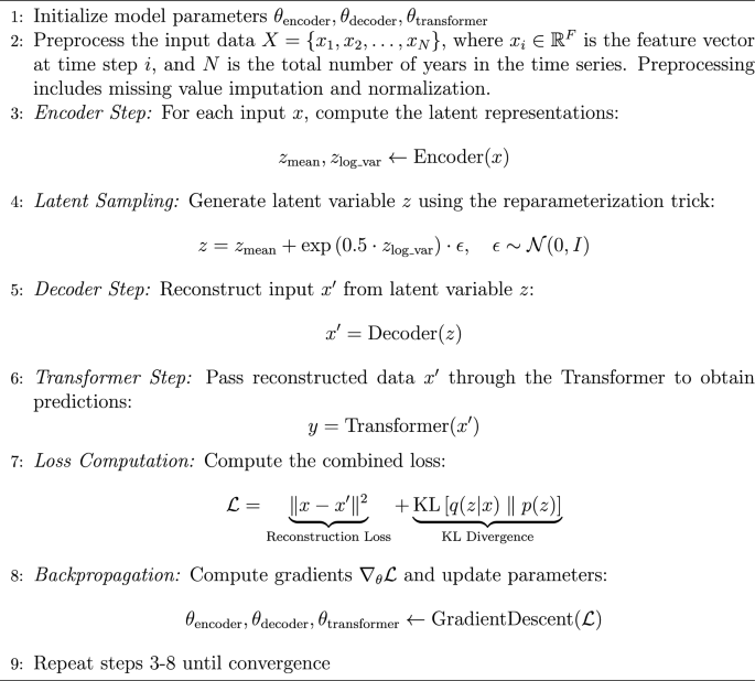
Training architecture of the transformer-VAE model, showing the encoder, latent space, and forecasting components.
The Transformer with VAE model excels particularly when dealing with missing or sparse data. The integration of the Transformer’s ability to capture long-term dependencies and the VAE’s capability to reconstruct missing values makes this model particularly robust37. By simultaneously learning temporal dependencies and generating synthetic data points, the model improves both its prediction accuracy and its robustness against noisy or incomplete data. This combination enhances the model’s ability to forecast future trends, even in situations where the data is incomplete or noisy, making it highly suitable for real-world applications involving sparse or missing data.
Long short-term memory (LSTM)
LSTM is a type of recurrent neural network (RNN) designed to model long-term dependencies in sequential data38. LSTM networks are equipped with gating mechanisms-specifically the input, forget, and output gates-that regulate the flow of information through the network39. This allows LSTM to selectively retain important information over time and discard irrelevant data, addressing the vanishing gradient problem encountered by traditional RNNs in long sequences40.
The state of the memory cell \(C_t\) and the hidden state \(h_t\) at each time step are updated as follows:
$$\begin{aligned} C_t = f_t \cdot C_{t-1} + i_t \cdot {\tilde{C}}_t\\ h_t = o_t \cdot \tanh (C_t) \end{aligned}$$
Where \(C_t\) is the memory cell at time step \(t\), representing the long-term memory of the model. \(h_t\) is the hidden state at time step \(t\), which contains the model’s output for the current time step. \(f_t\) is the forget gate, which decides how much of the previous memory cell \(C_{t-1}\) should be carried forward. \(i_t\) is the input gate, which controls how much of the candidate memory \({\tilde{C}}_t\) should be stored in the memory cell. \(o_t\) is the output gate, determining how much of the memory cell \(C_t\) should be output to the hidden state \(h_t\). \({\tilde{C}}_t\) is the candidate memory, which represents new information that could potentially be added to the memory cell. These gating mechanisms allow the model to effectively learn long-term dependencies and avoid issues like gradient vanishing, making LSTM well-suited for time-series forecasting and sequence modeling tasks.
The training of the LSTM network involves updating the model parameters through backpropagation over time. Algorithm 2 outlines the general steps for training an LSTM model:
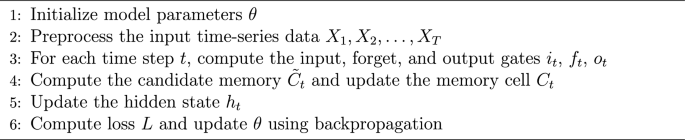
Training flow of the LSTM model for time-series forecasting of diabetes burden.
LSTM is particularly effective in tasks where long-term dependencies are crucial. A prime example is forecasting diabetes-related trends, where the progression of the disease is influenced by a variety of long-term factors such as medical history, lifestyle, and treatment regimens. LSTM’s ability to capture these complex temporal dependencies makes it an ideal model for predicting trends in chronic diseases, financial data, and other domains where historical context plays a significant role in forecasting future events41.
The LSTM model excels in capturing long-range temporal dependencies, making it highly effective for sequence modeling and time-series forecasting tasks. Its gating mechanisms ensure that relevant information is preserved over time while irrelevant data is forgotten, allowing for more accurate predictions over long sequences.
Gated recurrent unit (GRU)
The GRU is a variant of the LSTM network, designed to simplify the architecture while retaining the ability to model long-term dependencies in sequential data42. GRU combines the forget and input gates of LSTM into a single update gate \(z_t\), which controls the flow of information43. Additionally, the reset gate \(r_t\) is used to determine how much of the previous hidden state should be remembered when computing the candidate hidden state \({\tilde{h}}_t\)44.
The final hidden state \(h_t\) at each time step is computed as a weighted sum of the previous hidden state \(h_{t-1}\) and the candidate hidden state \({\tilde{h}}_t\), as shown in the following equation:
$$\begin{aligned} h_t = (1 – z_t) \cdot {\tilde{h}}_t + z_t \cdot h_{t-1} \end{aligned}$$
Where \(z_t\) is the update gate, determining how much of the previous hidden state \(h_{t-1}\) should be retained and how much of the candidate hidden state \({\tilde{h}}_t\) should be used to update the current hidden state. \(r_t\) is the reset gate, which controls the influence of the previous hidden state on the candidate hidden state \({\tilde{h}}_t\). \({\tilde{h}}_t\) is the candidate hidden state, calculated using both the input data and the reset gate, representing the potential new information for the current time step.
The GRU’s architecture allows it to model temporal dependencies with fewer parameters compared to LSTM, making it a computationally efficient model for many sequence-based tasks. Training a GRU network involves iteratively updating the model parameters using backpropagation through time (BPTT). Algorithm 3 outlines the general training procedure for a GRU model:
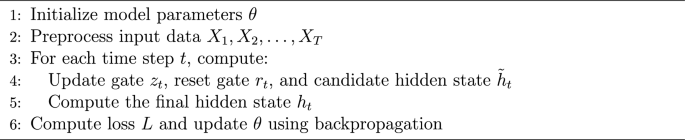
Training process of the GRU model, including sequence handling and prediction.
GRU models are particularly beneficial for sequence modeling tasks where computational efficiency is important, without sacrificing performance. For example, in applications such as time-series forecasting, speech recognition, and natural language processing, GRUs offer a simpler and faster alternative to LSTM, while still capturing essential temporal dependencies.
The GRU network is an effective alternative to LSTM that simplifies the gating mechanism while maintaining the ability to model long-range dependencies in sequential data. Its computational efficiency and simpler structure make it well-suited for real-time applications and resource-constrained environments.
Model training and hyperparameter optimization
Beyond dropout and batch normalization, additional regularization techniques were applied to further prevent overfitting. To mitigate overfitting due to limited sequence length per subgroup, we employed regularization techniques including dropout, KL annealing, and early stopping based on validation loss. L2 regularization (weight decay) was incorporated into the loss function to penalize excessively large model weights, enhancing generalization. Furthermore, hyperparameter tuning was conducted using a grid search approach to optimize key parameters, including learning rates, batch sizes, and layer configurations. These strategies collectively ensured the models maintained strong predictive performance while avoiding excessive reliance on training data, thereby improving their applicability in real-world forecasting scenarios.
To ensure a fair comparison, deep learning models underwent hyperparameter tuning via grid search, while ARIMA parameters were selected based on time-series diagnostics. The grid search procedure explored various combinations of hidden layers, attention heads, dropout rates, and learning rates to identify the most optimal settings. Mean Absolute Error (MAE) was used as the primary evaluation metric during hyperparameter tuning, ensuring that model configurations were optimized for predictive accuracy. The Adam optimizer was employed for deep learning models due to its adaptive learning capabilities. The final selected hyperparameters for each model are summarized in Table 2.
For ARIMA, preprocessing steps were applied to improve forecasting performance. The Augmented Dickey-Fuller (ADF) test was conducted to assess stationarity, and differencing was applied where necessary to transform non-stationary data into a stationary series. The optimal autoregressive order (p), differencing order (d), and moving average order (q) parameters were selected using Akaike Information Criterion (AIC) minimization, ensuring an optimal balance between model complexity and goodness of fit.
As ARIMA is inherently a univariate time series model, it cannot directly model multivariate inputs. Therefore, in this study, we applied separate ARIMA models to each health indicator-DALYs, deaths, and prevalence-independently. For each metric, we constructed and tuned an individual ARIMA configuration based solely on its historical time series within each income group. This allowed us to benchmark ARIMA’s predictive performance alongside multivariate deep learning models, while maintaining consistency in evaluation across indicators.
The Transformer-VAE model was configured with four encoder layers, each containing eight attention heads, and employed a dropout rate of 0.1 to prevent overfitting. The learning rate was set to 0.001 based on validation performance. The LSTM and GRU models were structured with two hidden layers of 128 units each, using a learning rate of 0.0005 and a dropout rate of 0.2 to enhance generalization. The ARIMA model’s parameters were determined dynamically through AIC minimization after ensuring stationarity with the ADF test.
Evaluation metrics
The performance of each model is evaluated using a comprehensive set of metrics, focusing on both prediction accuracy and computational efficiency, as well as the models’ ability to handle incomplete and variable data. The following metrics were used to assess model performance:
-
Prediction accuracy: The primary metric for evaluating prediction accuracy is the MAE, which measures the average absolute difference between the predicted and actual values. It is calculated as:
$$\begin{aligned} \text {MAE} = \frac{1}{n} \sum _{i=1}^n |y_i – {\hat{y}}_i| \end{aligned}$$
where \(y_i\) represents the actual values, \({\hat{y}}_i\) represents the predicted values, and \(n\) is the number of data points. A lower MAE indicates better accuracy in the model’s predictions. Additionally, we use Root Mean Squared Error (RMSE) to evaluate model performance by penalizing large errors more heavily. RMSE is calculated as:
$$\begin{aligned} \text {RMSE} = \sqrt{\frac{1}{n} \sum _{i=1}^n (y_i – {\hat{y}}_i)^2} \end{aligned}$$
RMSE provides a measure of how well the model captures deviations from the actual values, with larger values indicating poorer model performance.
-
Stability with variable data: The stability of the models is assessed by evaluating their ability to maintain prediction accuracy when exposed to changing trends in the data. A smaller accuracy drop indicates that the model is better at handling shifts in the data distribution, demonstrating its stability in the presence of evolving trends.
-
Stability analysis: This metric evaluates the model’s ability to maintain prediction accuracy across different conditions, including varying data characteristics. Stability is assessed by analyzing the residuals (the differences between predicted and actual values), with the goal of ensuring that these residuals remain small and consistent under different conditions. A model that demonstrates low variability in residuals is considered stable. We use the following residual analysis to measure stability:
$$\begin{aligned} \text {Residual} = y_i – {\hat{y}}_i \end{aligned}$$
where \(y_i\) is the actual value and \({\hat{y}}_i\) is the predicted value. The lower the spread of residuals, the more stable the model is.
-
Robustness to incomplete data: The ability of each model to handle missing or incomplete data is assessed using a combination of residual analysis and the model’s performance on datasets with missing values. The residuals from models trained on incomplete data are compared to those from models trained on complete data. Models that perform better with incomplete data are considered more robust. Specifically, we measure how well the model can adapt when missing values are introduced by calculating the increase in residuals:
$$\begin{aligned} \text {Residual Increase} = \frac{\sum _{i=1}^n |y_i – {\hat{y}}_i|_{\text {missing data}}}{\sum _{i=1}^n |y_i – {\hat{y}}_i|_{\text {complete data}}} \end{aligned}$$
A lower residual increase indicates better robustness to missing data.
-
Computational efficiency: The efficiency of the models is evaluated in terms of their computational cost. This includes three key aspects:
-
Training time: The time taken to train the model on the training dataset, typically measured in minutes or seconds.
-
Inference time: The time taken by the model to make predictions on unseen test data, measured in seconds.
-
Memory usage: The amount of memory consumed by the model during both training and inference phases, typically measured in megabytes.
We aim to balance accuracy with efficiency, with a model that performs well but also operates within reasonable computational limits.
-
By evaluating these metrics, we gain a comprehensive understanding of how well each model performs not only in terms of prediction accuracy but also in terms of computational efficiency, robustness to missing data, and stability under varying conditions.