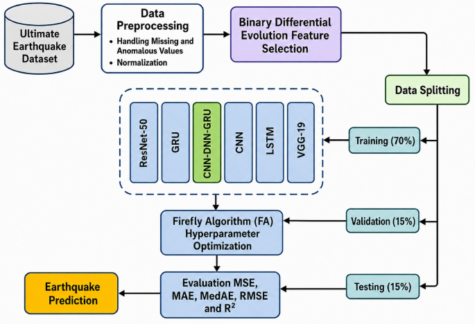
This paper proposes a hybrid deep learning framework, CNN–DNN–GRU, for earthquake magnitude estimation, optimized using Binary Differential Evolution (BDE) for feature selection and the Firefly Algorithm (FA) for hyperparameter tuning. The raw dataset comprises 3,500,000 global seismic-event records spanning 1990–2023.The data were preprocessed by handling anomalous values, constructing chronological event-history sequences, and partitioning the resulting sequences chronologically into 70% training, 15% validation, and 15% testing subsets. Normalization parameters were estimated exclusively from the training subset and subsequently applied to the validation and test subsets. BDE was employed to identify the most informative features, reducing redundancy and improving model efficiency. The hybrid model architecture combines a CNN for spatial feature extraction, a DNN for capturing complex nonlinear relationships, and a GRU for learning temporal dependencies. FA was used to optimize key hyperparameters such as learning rate, number of neurons, dropout rate, and GRU units by minimizing the validation error. The model was trained using the Adam optimizer and evaluated using standard regression metrics including MAE, RMSE, MAPE, and \(R^2\). Its performance was benchmarked against baseline models, including CNN, LSTM, GRU, ResNet50, and VGG-19, to demonstrate its predictive superiority and robustness. Figure 1 illustrates the framework of the proposed methodology for earthquake magnitude estimation.

The proposed hybrid model for earthquake magnitude estimation.
Dataset
To develop and evaluate the proposed CNN-DNN-GRU earthquake magnitude estimation model, a comprehensive seismic dataset was utilized, sourced from The Ultimate Earthquake Dataset (1990–2023) available on44. This dataset aggregates global seismic activity over more than three decades, offering a rich, diverse collection of earthquake records with essential geophysical parameters. The dataset comprises 3,500,000 instances, each representing a unique earthquake event, and includes the following seven primary features as detailed in Table 1. Notably, the target variable for our prediction framework, ’magnitude’, represents the Moment Magnitude (Mw) scale, the standard measure of the strength of these seismic events.
It is important to distinguish between independent input variables and target-derived or post-event descriptors. Although the raw dataset contains the significance variable, this feature was excluded from the final predictive input space. The significance score is strongly associated with earthquake magnitude and may also incorporate post-event impact-related information, such as felt reports, damage, casualties, or economic consequences. Therefore, it may not be available before or during the initial magnitude-estimation stage in real applications. Using this variable as an input for predicting magnitude would create a risk of information leakage and recursive prediction, where information partly derived from the target is used to estimate the target itself.
For this reason, significance was retained only for exploratory data analysis and descriptive visualization, but it was not used in model training, validation, testing, BDE-based feature selection, or FA-based hyperparameter optimization. The final leakage-free input space was restricted to independent earthquake-event metadata that are not directly derived from the target magnitude.
To provide complete transparency about the nature of the data and to explicitly demonstrate the information available to the model, Table 2 presents a typical row from the raw dataset CSV file. This example clarifies that the dataset consists solely of tabular point-in-time metadata describing the earthquake’s core parameters and confirms that no time-series ground-motion records or waveform severity measures were used.
Table 3 presents the Statistical analysis of the raw earthquake dataset before preprocessing, which consists of 3,500,000 earthquake records, with seven features analyzed for their distributions. The magnitude feature has a mean of 1.97 and ranges from −9.99 to 8.40, indicating the presence of outliers or missing values encoded as negative values. Depth ranges from −10 km to 712.5 km, with a mean of 20.3 km, capturing shallow- to deep-focus earthquakes. It is important to note that in standard seismological catalogs, depth is measured relative to mean sea level; therefore, valid negative depth values indicate events occurring above sea level in elevated mountainous or volcanic regions. Latitude and longitude values confirm global coverage, spanning from −83.9° to 87.1° and −179.9° to 180°, respectively. The significance score, which reflects the event’s impact, shows high variability, with a maximum of 1,750. The status field is predominantly constant with a mean near 3.0, indicating uniform processing. Finally, the tsunami feature is consistently zero, suggesting no tsunami-triggered events are labeled in this dataset.
Figure 2 displays a correlation heatmap that visualizes the linear relationships among the dataset’s numerical features. Notably, magnitude and significance exhibit a robust positive correlation (0.95), suggesting that as magnitude increases, the earthquake’s importance also rises. Magnitude also shows moderate positive correlations with longitude (0.61) and depth (0.38), and a negative correlation with latitude (−0.47). The significance feature similarly correlates with depth (0.40) and longitude (0.66), but negatively with latitude (−0.51).

Correlation heatmap of key seismic features.
The density plots in Figure 3 provide insight into the distribution of each feature within the earthquake dataset. The status and tsunami variables are highly imbalanced, with most records showing a constant value (status 3, tsunami = 0), indicating little to no variability. Significance, depth, and magnitude are right-skewed, with most events having low values and fewer high-impact events. Specifically, magnitude clusters between 0 and 5, while depth and significance peak at lower values and taper off toward the extreme ends. The longitude and latitude distributions are more complex, showing multimodal patterns that reflect the global spread of seismic activity, with notable peaks corresponding to seismically active regions.

Density distribution plots of dataset features.
The scatter matrix in Figure 4 shows the relationship between numerical features in a dataset, revealing skewed distributions and moderate positive correlations. It also reveals global coverage, broad distributions of longitude and latitude, and sparse distributions of features such as status and tsunami.

Scatter matrix plot of earthquake dataset features.
Boxplots in figure 5 show the central tendency, dispersion, and presence of outliers in the earthquake dataset—magnitude, significance, and depth —indicating rare but high-impact seismic events. Latitude and longitude show a wide interquartile range.

Boxplot visualization of each feature, highlighting value distribution, presence of outliers, and skewness across key seismic parameters in the dataset.
The histogram plots in Figure 6 provide a detailed view of the frequency distributions of the earthquake-dataset features. The status and tsunami variables are highly imbalanced, while significance, magnitude, and depth exhibit strongly skewed distributions. Latitude and longitude show broader and multimodal distributions reflecting the global spatial distribution of seismic activity. In particular, the depth distribution is strongly right-skewed, with most earthquake events occurring at relatively shallow depths and progressively fewer events occurring at greater depths.

Histogram plots of seismic dataset features, illustrating the frequency distributions, skewness, and dominant value ranges across key earthquake parameters.
Data preparation
Data preprocessing is a critical step to ensure data quality and compatibility with the deep learning model. The raw dataset, containing 3,500,000 event instances and seven features, underwent the following steps:
-
Handling Missing and Anomalous Values: The raw earthquake catalog contained 3,500,000 event records spanning 1990–2023. As shown in Table 3, all reported variables contained 3,500,000 observations; therefore, no conventional missing or NaN values were identified, and no records were removed because of missing data. The raw magnitude values ranged from \(-9.99\) to 8.40. Negative magnitudes were not removed indiscriminately because small negative magnitudes may represent physically valid low-energy microseismic events. However, the specific value \(M=-9.99\) was treated as an invalid catalog placeholder rather than a physically meaningful earthquake magnitude. A total of 57,974 records satisfying this criterion were removed, corresponding to 1.6564% of the original dataset. Other negative magnitude values were retained. The hypocentral-depth values ranged from \(-10\) to 712.5 km. Negative depth observations were not considered invalid solely because they were below zero, because earthquake-catalog depths may be referenced to mean sea level and slightly negative values may occur for shallow events in elevated regions or because of hypocentral-location uncertainty. Consequently, no records were removed solely on the basis of a negative depth value. Following these record-level validity checks, 3,442,026 valid earthquake-event records remained. The subsequent removal of significance, status, and tsunami from the predictive input represents feature-level screening rather than record-level deletion. Significance was excluded because of its strong association with the target magnitude and the resulting risk of information leakage, whereas status and tsunami were excluded because of their negligible variability. The final leakage-free input variables were therefore longitude, latitude, and depth. As summarized in Table 4, the data-quality screening reduced the original 3,500,000 earthquake-event records to 3,442,026 valid observations. No records were removed because of conventional missing values or solely because of negative hypocentral depth. Record-level exclusion was primarily associated with the invalid magnitude placeholder \(M=-9.99\), which accounted for 57,974 observations (1.6564% of the original dataset). In contrast, the exclusion of significance, status, and tsunami was performed at the feature level and did not further reduce the number of earthquake events. This distinction ensures that potentially meaningful low-energy and shallow seismic events are retained while invalid target values and leakage-prone or uninformative features are excluded.
Table 4 Summary of the data-cleaning and feature-screening procedure. -
Normalization: All numerical features were scaled to the range [0,1] using Min-Max normalization, defined in eq 1:
$$\begin{aligned} x’ = \frac{x – x_{\min }}{x_{\max } – x_{\min }} \end{aligned}$$
(1)
Where \(x\) is the original feature value, \(x_{\min }\) and \(x_{\max }\) are the minimum and maximum values of the feature in the dataset, and \(x’\) is the normalized value.
-
Categorical Encoding: The ’status’ feature was label-encoded. However, given its lack of variability, it was considered non-essential and excluded from final modeling.
-
Data Splitting: To preserve the temporal structure of the earthquake catalog and prevent information leakage, random partitioning was not employed. After the earthquake records were ordered by event time and the chronological sequences were constructed, the resulting samples were divided chronologically into 70% training, 15% validation, and 15% testing subsets. The earliest 70% of the sequences were assigned to the training set, the subsequent 15% to the validation set, and the most recent 15% to the independent test set. This procedure ensures that information from future earthquake events is not available during model training or validation.
Temporal sequence construction for GRU input
Although the raw earthquake catalog consists of point-wise tabular event records, the GRU component requires sequential input. Therefore, before training the CNN–DNN–GRU model, the catalog records were transformed into chronological event-history sequences. First, all earthquake records were ordered according to their event time. Then, a fixed-length sliding-window strategy was applied to construct sequential samples from previous events.
In this study, the sequence length was set to \(L=10\). This means that each input sample contains the leakage-free metadata of the previous ten earthquake events, and the target output is the magnitude of the following event. For a given time step \(t\), the input sequence is defined as:
$$\textbf{S}_{t} = [\textbf{x}_{t-10}, \textbf{x}_{t-9}, \ldots , \textbf{x}_{t-1}]$$
where \(\textbf{x}_{t}\) denotes the leakage-free feature vector of the \(t\)th earthquake record. The corresponding target is:
where \(M_t\) is the magnitude of the following earthquake event.
To avoid target leakage, variables derived from magnitude or post-event impact, such as significance, were excluded before sequence construction. Constant or weakly informative variables, such as status and tsunami, were also excluded from the final modeling input. Therefore, each event vector contains three independent metadata features:
$$\textbf{x}_t = [longitude_t, latitude_t, depth_t]$$
Accordingly, the input tensor provided to the CNN–DNN–GRU model has the shape:
where \(N\) is the number of constructed samples, 10 is the number of previous events in each sequence, and 3 is the number of leakage-free input features.
To prevent temporal information leakage, no random train–validation–test partitioning was performed. After chronological ordering and sequence construction, the resulting samples were divided according to event time into 70% training, 15% validation, and 15% testing subsets. Specifically, the earliest 70% of the sequences were used for model training, the subsequent 15% were used for validation, BDE-based model selection, and FA-based hyperparameter optimization, and the most recent 15% were retained as an independent test set and were not involved in any training or optimization stage. Furthermore, the normalization parameters were estimated exclusively from the training subset and subsequently applied unchanged to the validation and test subsets. This chronological evaluation protocol preserves the temporal ordering of the earthquake catalog and ensures that information from future events is not used to predict earlier events.
BDE objective function for feature selection
Binary Differential Evolution (BDE) was adopted as a wrapper-based feature-selection method to identify the most informative subset of seismic input variables for earthquake magnitude estimation. In this framework, each BDE individual represents a binary feature-selection vector:
$$\begin{aligned} \textbf{z}_i = [z_{i1}, z_{i2}, \ldots , z_{id}] \end{aligned}$$
(2)
where d is the total number of input features, and \(z_{ij} \in \{0,1\}\) indicates whether the jth feature is selected. A value of \(z_{ij}=1\) means that the feature is retained, whereas \(z_{ij}=0\) means that the feature is excluded from the model input.
The BDE search process was guided by a wrapper-based objective function that considers both prediction error and feature-subset compactness. The fitness value of each candidate feature subset was computed as:
$$\begin{aligned} Fitness(\textbf{z}_i) = \lambda \times MSE_{val}(\textbf{z}_i) + (1-\lambda ) \times \frac{\sum _{j=1}^{d} z_{ij}}{d} \end{aligned}$$
(3)
where \(MSE_{val}(\textbf{z}_i)\) denotes the validation mean squared error obtained using the selected feature subset, \(\sum _{j=1}^{d} z_{ij}\) represents the number of selected features, d is the total number of available features, and \(\lambda\) is a weighting coefficient used to balance prediction accuracy and feature reduction.
In this study, prediction accuracy was given higher priority than feature reduction; therefore, \(\lambda\) was set to a high value. This allows BDE to primarily minimize the validation error while still discouraging unnecessarily large feature subsets. Accordingly, the BDE algorithm optimizes two selection criteria: (i) minimizing earthquake magnitude prediction error and (ii) reducing redundant or weakly informative input variables. Mutual information was not used as the main selection criterion because the aim of this study is to select features that directly improve the regression performance of the proposed CNN–DNN–GRU model. The final selected subset was the feature mask with the lowest fitness value on the validation subset.
BDE feature-selection results
To demonstrate the contribution of Binary Differential Evolution (BDE), the selected feature subset was explicitly reported after preprocessing and leakage-control screening. Since the magnitude variable represents the target output and significance may introduce target leakage, these variables were not included in the BDE input space. In addition, variables with limited variability, such as status and tsunami, were excluded before model training. Therefore, BDE was applied to the final leakage-free candidate feature set consisting of longitude, latitude, and depth.
Each BDE individual was represented as a binary mask, where 1 indicates that the feature is selected and 0 indicates that the feature is excluded. The selected feature subset was determined by minimizing the wrapper-based fitness function defined in the previous subsection, which combines validation MSE and a feature-size penalty. Table 5 presents the final BDE-selected features.
The BDE output shows that longitude, latitude, and depth were retained as the final leakage-free input features. Longitude and latitude provide spatial-context information related to regional tectonic setting, while depth provides hypocentral information that may influence magnitude estimation. However, these variables are interpreted as catalog-level descriptors rather than direct causal predictors of earthquake magnitude.
CNN–DNN–GRU hybrid model architecture
The proposed CNN–DNN–GRU hybrid model is shown in Figure 7, which integrates convolutional, dense, and recurrent layers to effectively capture spatial, abstract, and temporal patterns from earthquake-related input data.
The architecture begins with two one-dimensional convolutional layers, each using 32 filters, a kernel size of 3, and ReLU activation, followed by a max-pooling layer with pool size = 2 and a dropout layer with a rate of 0.2 to reduce overfitting. The use of kernel_size=3 is consistent with the Conv1D operation, where the convolutional kernel is applied along one input dimension. Algorithm 1 displays the CNN-DNN-GRU hybrid model.

CNN-DNN-GRU architecture.
To clarify the design of the recurrent component, the first GRU layer was configured with return_sequences=True because its role is to preserve the complete learned temporal representation and pass the full sequence of hidden states to the following GRU layer. This allows the second GRU layer to further refine the sequential dependencies extracted from the CNN feature maps. In contrast, the second GRU layer was configured without returning sequences because the target task is a single-output regression problem, where the model estimates one earthquake magnitude value for each input sample. Therefore, the final hidden state of the second GRU layer provides a compact temporal summary that is suitable for the subsequent dense regression block.
A bidirectional GRU was not adopted in the proposed architecture for two main reasons. First, the intended application is earthquake magnitude estimation in a forecasting or early-warning-oriented setting, where future temporal context may not be available at inference time. Bidirectional recurrent layers process the input in both forward and backward directions and may therefore rely on information that would not be accessible in a real-time scenario. Second, the dataset used in this study consists of tabular earthquake-event metadata rather than continuous raw waveform sequences; therefore, using a bidirectional or full sequence-output recurrent structure may unnecessarily increase the number of trainable parameters, computational complexity, and overfitting risk. For this reason, the adopted two-layer GRU design provides a practical balance between temporal representation learning, model simplicity, and regression-oriented output generation.

Coupling strategy between BDE and FA
The proposed optimization framework couples BDE and FA in a sequential manner rather than an alternating or co-evolutionary manner. In the first stage, BDE is applied for feature selection. Each BDE individual represents a binary feature mask, where a value of 1 indicates that the corresponding feature is selected and a value of 0 indicates that it is excluded. The objective of this stage is to identify the most informative feature subset that minimizes prediction error while reducing redundant or weakly informative variables.
After the BDE process is completed, the selected feature subset is fixed and transferred to the second optimization stage. In the second stage, FA is used to tune the hyperparameters of the CNN–DNN–GRU model, such as the learning rate, dropout rate, number of GRU units, and number of dense neurons. Thus, the information transfer between BDE and FA is one-directional: BDE provides the selected feature mask to FA, while FA optimizes the model hyperparameters using only these selected features. FA does not modify the BDE-selected feature subset, and BDE is not re-executed during FA iterations.
This sequential coupling strategy was adopted for three reasons. First, performing feature selection before hyperparameter tuning reduces the dimensionality of the input space and removes redundant variables before model optimization. Second, fixing the selected feature subset before FA optimization reduces the computational burden because FA evaluates candidate neural-network configurations on a reduced feature space. Third, separating feature selection and hyperparameter tuning improves the stability and interpretability of the optimization pipeline, since the contribution of each stage can be clearly identified. Therefore, the proposed BDE–FA coupling can be summarized as follows:
$$\textbf{X}_{raw} \xrightarrow {\textrm{BDE}} \textbf{X}_{selected} \xrightarrow {\textrm{FA}} \theta ^{*}_{CNN-DNN-GRU} \xrightarrow {\textrm{Training}} \hat{y}$$
where \(\textbf{X}_{raw}\) denotes the original input feature matrix, \(\textbf{X}_{selected}\) denotes the BDE-selected feature subset, \(\theta ^{*}_{CNN-DNN-GRU}\) represents the optimal hyperparameter configuration obtained by FA, and \(\hat{y}\) is the predicted earthquake magnitude.
Firefly algorithm for hyperparameter optimization
In the proposed CNN–DNN–GRU model, the Firefly Algorithm (FA) is adopted as a metaheuristic strategy to optimize critical hyperparameters and enhance model performance. The FA simulates the natural flashing behavior of fireflies, in which less-bright fireflies move toward brighter ones, based on an attractiveness function that decreases with distance and is modulated by a light-absorption coefficient. Each firefly in the population encodes a candidate solution representing a combination of hyperparameters such as learning rate, dropout rate, and the number of units in GRU and dense layers. The brightness of each firefly is determined by the validation loss (e.g., mean squared error) obtained during training with the corresponding configuration. Through iterative updates influenced by attractiveness and random perturbations, the FA effectively explores the search space to locate optimal configurations. This approach significantly improves the convergence rate, generalization, and predictive accuracy of the proposed model for earthquake magnitude forecasting. Algorithm 2 displays the FA hyperparameter optimization method.
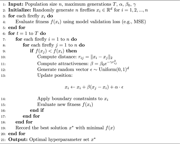
FA for Hyperparameter Optimization.
To avoid ambiguity regarding the role of the validation set during FA optimization, the data partitioning strategy was strictly fixed before the optimization process. The dataset was first divided into three mutually exclusive subsets: training, validation, and testing. For each firefly, the encoded hyperparameter configuration was used to train the CNN–DNN–GRU model only on the training subset. The validation subset was then used to compute the fitness value, defined as the validation mean squared error (MSE), as follows in eq 4:
$$\begin{aligned} Fitness(x_i) = MSE_{val}(x_i) = \frac{1}{N_{val}}\sum _{k=1}^{N_{val}}(y_k-\hat{y}_k)^2 \end{aligned}$$
(4)
where \(x_i\) denotes the hyperparameter vector represented by the ith firefly, \(N_{val}\) is the number of validation samples, \(y_k\) is the actual magnitude, and \(\hat{y}_k\) is the predicted magnitude. The validation subset was used only for model selection and was not used for gradient-based weight updates. The independent test subset was kept completely unseen during training, BDE-based feature selection, and FA-based hyperparameter optimization, and it was used only once for the final evaluation of the selected model.
Nevertheless, using the same validation subset repeatedly during the FA search may still introduce validation-set selection bias, particularly when the number of evaluated configurations is large. To reduce this risk, the search space was constrained to a limited number of meaningful hyperparameter ranges, and the final model was evaluated on an independent test set that did not participate in any optimization step. In future work, nested cross-validation and repeated independent train–validation–test splits will be adopted to further reduce optimizer-induced overfitting and provide a more robust estimate of generalization performance.
Although the FA is used to optimize the hyperparameters of the proposed CNN–DNN–GRU model, it is important to note that the FA itself contains several control parameters, including the population size, maximum number of generations, randomization factor \(\alpha\), base attractiveness \(\beta _{0}\), and light absorption coefficient \(\gamma\). These parameters affect the balance between exploration and exploitation during the optimization process. In this study, the FA control parameters were selected based on commonly adopted ranges in previous metaheuristic optimization studies and refined through preliminary validation experiments. The final configuration was chosen according to the lowest validation MSE, while the independent test set was kept unseen until the final evaluation stage. Therefore, the selected optimizer parameters are not claimed to be universally optimal; rather, they represent empirically effective settings for the present earthquake magnitude estimation task. This validation-based selection strategy reduces the risk of test-set bias and provides a practical balance between optimization performance and computational cost. Similarly, the BDE parameters used for feature selection were selected to maintain sufficient population diversity while ensuring convergence within a reasonable computational budget. Since metaheuristic algorithms are stochastic by nature, their performance may vary depending on initialization and control-parameter settings. To reduce this effect, the optimization process was repeated, and the best feature subset was selected based on validation performance rather than final test performance. This procedure ensures that feature selection is guided by generalization behavior instead of direct fitting to the test set.
Implementation details and reproducibility
Table 6 displays Implementation and reproducibility details such as The deep learning models were developed using TensorFlow 2.10 and Keras 2.10, while the machine learning baselines were implemented using Scikit-learn 1.1.3.