Quantifying global migration
Current methods for estimating global migration rely on relatively straightforward techniques compared with the advanced computational approaches adopted in recent years for predicting and explaining human migration and mobility. Estimates of global migrant population stocks, by country of birth and country of residence, are derived from official statistics on foreign-born or foreign populations, with simple interpolation across census years and imputation when data are missing or inconsistent, using regional averages, demographic assumptions or alignment with changes in the population totals22.
The availability of migration flow data is much more limited than that on migrant stocks. Countries that publish migration statistics tend to have well-developed statistical infrastructure for monitoring population movements located in rich, developed settings. The scale of migration flows occurring between developing countries and to and from some of the world’s most populous nations is often unknown. Consequently, to estimate origin-destination migration flows at the global level, indirect methods have been developed based on changes in global migrant stock estimates. These methods were reviewed in a previous work9, alongside a systematic comparison. They identified six methods, grouping them into three classes.
The first class comprises two stock-differencing approaches, which treat changes in bilateral migrant stocks between census rounds as flows. Negative differences are either set to zero or interpreted as return migration. The second class is a migration-rate approach, which derives transition rates directly from a single stock table by dividing each off-diagonal stock count by the global foreign-born population. These rates are then scaled by an approximation of the total number of global flows, calculated as the sum of absolute net migration flows.
The third class includes three demographic accounting methods, which reconcile changes in birth-place-destination stocks, total population, births and deaths with estimated origin-destination flows. In this framework, adjusted stock tables at the beginning and end of the period are used to define outflow and inflow margins. These margins are then arranged into a three-way array of origin, destination and birthplace flows. Missing values in this array are imputed so that the reconstructed flow table matches the stock-based margin totals. To achieve this, an iterative proportional fitting algorithm, adapted from a past work73, is applied to adjust the cell values until the row, column and diagonal constraints are satisfied. Variants of this framework differ in whether inconsistencies in inflow and outflow margins are absorbed into an open demographic system by introducing a residual category12 or resolved in a closed demographic system by scaling adjusted stock tables to enforce consistency13. A further extension combines two imputation strategies within the closed demographic accounting system by weighting alternative treatments of the diagonal cells in the array that represent non-migrants14. The first imputation sets the diagonals to their maximum feasible values, whereas the second applies an independent log-linear fit that relaxes this constraint. The final flow estimates are obtained as a weighted average of the two imputations, with weights calibrated against harmonized European migration flow data. Although each method has trade-offs, the weighted demographic accounting approach produced estimates that were most consistent with reported flow statistics in countries with official data9.
All applications of these indirect methods are constrained by the temporal spacing of the available migrant stock data, typically five-year intervals, and by errors or inconsistencies in the underlying stock statistics. As a result, the estimated flows inherit the limitations of the stock data, including inaccuracies in imputations by UN DESA or other agencies, which can affect both the precision and comparability of global migration flow estimates. Moreover, these methods make use of very limited covariate information—only allowing information via a single variable for the seed values of the iterative proportional fitting procedure, which has minimal impact—further restricting their ability to capture corridor-specific dynamics or explanatory factors.
More recently, direct estimates of global migration flows have been produced using large-scale online data sources21 (discussed above). The estimates represent a substantial advance over indirect methods, as they are based on observed movements, provide higher temporal resolution, and avoid relying solely on changes in migrant stock data. However, the data cover only a limited number of years, omit several important countries, and will not be updated, restricting their long-term utility.
Recurrent neural network approach to quantifying global migration
Demographic account for global migration estimation
UN DESA provides estimates of global migrant stock Sbi(t), that is, the number of people born in country b living in country i at time t (ref. 22). These data are given at five-year intervals from 1990 to 2020, as well as a recent estimate for 2024. The stocks evolve deterministically according to the equation
$${\partial }_{t}{S}_{bi}
(2)
where Bi and γi are, respectively, the total number of births and the mortality rate of the country of residence, and δbi is the Kronecker matrix
$${\delta }_{bi}=\left\{\begin{array}{ll}1, & {\rm{if}}\,b=i,\\ 0, & {\rm{e}}{\rm{l}}{\rm{s}}{\rm{e}}.\end{array}\right.$$
(3)
The first term in equation (2) simply means that all births in a country increase the native-born stock Sii; the second models population decrease due to deaths; the third models the change in stocks due to migration. Tbij is the flow of migrants born in b from country i to j, and is the quantity we wish to infer. The total flow of people from i to j, regardless of their place of birth, is of course then given by
$${F}_{ij}=\sum _{b}{T}_{bij},$$
(4)
while a country’s net migration (arrivals minus departures) is
$${{\bf{M}}}_{i}=\sum _{j}{F}_{ji}\,-\,{F}_{ij}.$$
(5)
Target data
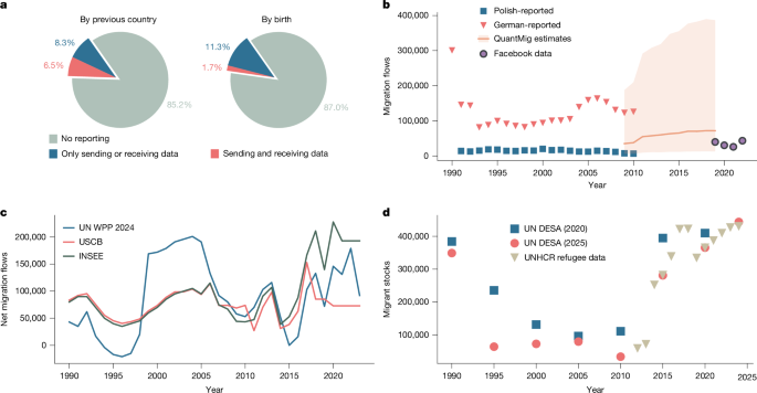
Aside from the stock data, there are numerous datasets of partial observations of the flow F and the net migration \({\bf{M}}\) to which we could constrain our estimate \(\hat{T}\), although, as mentioned in the introduction, these do not always use consistent definitions of a migration event. The UN DESA World Population Prospects dataset53 and the US Census Bureau International Database70 both provide estimates of annual net migration for all countries from 1950 to 2024. These figures are mainly calculated as the residual between the total change in population and natural growth (births minus deaths), and for most countries, they are not derived from immigration statistics; we thus do not include them as target variables. Instead, we use net annual migration statistics from around 30 countries and territories in Europe, North America, Oceania and East Asia, sourced from national statistical bureaus (Supplementary Information).
Observations of total origin-destination flows F are taken mainly from five sources, which all use a one-year definition of migration flows:
-
Harmonized intra-European flows: the QuantMig database10,11 provides probabilistic estimates of migration flows between 30 countries in Europe from 2009 to 2019, and is based on publicly available Eurostat data. These have been harmonized to use a common definition of migration, and also provide uncertainty estimates, which we use to weight the target data points in the loss function used to train the neural network (see below).
-
National immigration statistics from Sweden, New Zealand and Finland74,75,76: all three countries report total annual in- and out-flows by origin and destination.
-
Facebook data21: estimates of annual bilateral migration flows between 181 countries from 2019 to 2022 from an analysis of online social media data. We only include annual flows of at least 25 people, as noise was added by the authors to prevent data disclosure, which distorts small values.
Target values are prioritized in this order, meaning that if two datasets both contain values for the same origin–destination pair, we use the source furthest up in the list.
Input covariates
Each value Tbij is a flow through a network multi-edge connecting the birth country b, the origin i and destination j. We train a deep neural network to learn a mapping \({{\boldsymbol{\chi }}}_{bij}
(6)
Note that the estimates \({\widehat{T}}_{bij}\) and all their derived quantities will be real-valued, despite integer target data. This gives a recursive training procedure, where each output is fed back into the neural network to inform the next estimate (Extended Data Fig. 1a). The latent state zbij is initialized at zero and can take any value in \({{\mathbb{R}}}^{Z}\).
The neural network consists of a set of trainable parameters θ that are optimized using the gradient of the loss function, J, which is designed to ensure that predicted and observed stocks, net migration values and flows Fij agree, and is structurally an L2-loss of all of the different values {yk}. We make two important modifications to this basic loss function: first, we scale the data to make the errors \(\widehat{y}-y\) more normal, ensuring the loss function is not dominated by the largest values (this will be addressed below); and second, we weight each term in the loss function by its uncertainty to bias the loss towards values in which we have greater confidence (Extended Data Fig. 1c):
$${J}_{\theta }\approx \sum _{k}{w}_{k}{({\widehat{y}}_{k}-{y}_{k})}^{2},$$
(7)
with the index k ranging over all of the target values in a single batch. The weights wk are constructed from the relative uncertainty on each point, clamped to the interval [0.5, 2], and normalized such that the mean weight is 1. The QuantMig dataset provides standard errors on the estimates which we use to populate the weights for the flow targets; for all other flow targets, we set the weight to the average weight of the QuantMig weights or 1. For the stocks, we apply the demographic accounting scheme presented in past works9,12: given the stock tables for two successive years S(t1), S(t2), we add births and deaths, and constrain the resulting tables to match their midpoint marginals using iterative proportional fitting. Subsequently subtracting births and deaths again gives two demographically balanced stock estimates for each year, from which we can estimate the uncertainty on each value Sbi. For the net migration targets, we set the weights to 1 (refer to the Supplementary Information for details).
Scaling the input and target data
Much of the input and target data are heavily skewed Poisson distributions, with long tails caused by a small number of strong outliers; to improve learning, it is common practice to transform data to make it more normal. To this end we use a symmetrized Yeo–Johnson transform:
$${\psi }_{\lambda }(x)={\rm{s}}{\rm{g}}{\rm{n}}(x)\times \left\{\begin{array}{l}\frac{{(| x| +1)}^{\lambda }\,-\,1}{\lambda }\,{\rm{i}}{\rm{f}}\,\lambda \ne 0,\\ \log (| x| +1)\,{\rm{e}}{\rm{l}}{\rm{s}}{\rm{e}}\end{array}\right.$$
(8)
with \({\rm{s}}{\rm{g}}{\rm{n}}(x)\) the sign function. Compared with the standard transformation92, the symmetrization ensures that negative values are transformed more evenly. The parameter λ can be chosen to move the distribution of ψλ(x) closer towards a normal distribution (Extended Data Fig. 1b); for λ = 1, ψ is simply the identity. The transformed input data are further normalized to have zero mean and unit variance. Note that the transformation equation (8) is invertible, with inverse \({\psi }_{\lambda }^{-1}\); we can thus always reverse any transformation to obtain the original data. We rescale all non-binary covariates except the religious and linguistic similarity indices to be approximately normal (refer to the Supplementary Information for the λ values used for each).
To improve prediction accuracy on edges with smaller flows, we also transform the target data using the above function ψ; the loss function then reads
$$\begin{array}{c}{J}_{\theta }\,=\,\langle {w}_{bi}^{s}{({\psi }_{{\lambda }_{1}}(\Delta {\hat{S}}_{bi})-{\psi }_{{\lambda }_{1}}(\Delta {S}_{bi}))}^{2}\rangle \\ \,+\,\langle {w}_{i}^{m}{({\psi }_{{\lambda }_{2}}({\hat{{\bf{M}}}}_{i})-{\psi }_{{\lambda }_{2}}({{\bf{M}}}_{i}))}^{2}\rangle \\ \,+\,\langle {w}_{ij}^{f}{({\psi }_{{\lambda }_{3}}({\hat{F}}_{ij})-{\psi }_{{\lambda }_{3}}({F}_{ij}))}^{2}\rangle .\end{array}$$
(9)
Here, ⟨⋅⟩ denotes the average over all target values. Observe that we are not matching stock values directly, but rather the difference in stocks over five-year intervals. This is to avoid conditioning the stock value on (possibly erroneous) initial values, and ensure independence of the stock estimates. An optimal initial stock value can be estimated after training using a least squares approach, to fit the time series \({\widehat{S}}_{bi}
(10)