Deep learning-based profiling side-channel attacks in SPECK cipher

Notation

Calligraphic letters \(\mathscr {X}\) represent sets and where the calligraphic letter is finite, \(|\mathscr {X}|\) will represent the cardinality of \(\mathscr {X}\). X denote random variables and random vectors X over \(\mathscr {X}\). Consequently, x and x represent the realizations of X and X, respectively. Thus, the i-th entry of the vector x is \({{{\textbf {x}}}_i}\). For each entry, \({{{\textbf {x}}}_i}\), there is an associated key candidate and plaintext bytes. Thus, let k be a key candidate, with possible values in key space \(\mathscr {K}\). From this key space, \(k^{*}\) denotes the correct key. Therefore, the key guess associated with \({{{\textbf {x}}}_i}\) is \(k_i\) and likewise the associated plaintext is \(PT_i\).

Profiling side-channel attack

Embedded devices unintentionally emit physical information, such as power consumption, electromagnetic radiation, and timing delays, as a byproduct of processing cryptographic data²⁴. Side-channel attacks exploit these leakages to extract sensitive information, such as cryptographic keys, bypassing the mathematical security of the cryptographic algorithms by targeting their physical implementations. These attacks when categorized based on the exploited leakage channels, include timing attacks, electromagnetic radiation attacks, acoustic attacks, and power analysis attacks, all of which pose significant security risks to cryptographic systems.

Furthermore, side-channel attacks can be classified based on the level of knowledge an attacker has about the target device. The two primary categories are non-profiling attacks and profiling attacks. In non-profiling attacks, the attacker aims to uncover the secret key of a target device by analyzing side-channel measurements gathered from multiple encryption operations using different plaintexts. The adversary exploits the correlation between certain key-dependent intermediate values and the observed physical leakages. This method is commonly employed in techniques such as Differential Power Analysis (DPA) and Correlation Power Analysis (CPA), where statistical tools are used to link leakage patterns to cryptographic key information.

On the other hand, in profiling attacks, the attacker possesses a clone device that they can use to characterize leakages, thus effectively representing the dependency relation between the secret key and side-channel information. The presence of a clone device in profiling attacks inadvertently positions the adversary as more powerful compared with non-profiling attacks. The adversary might require hundreds of thousands of measurements to build a profiling model to characterize the side-channel leakage, making profiling attacks the worst-case scenario for security analysis. Therefore, our proposed method in this work is based on profiling side-channel analysis. We will establish the two phases of profiling attacks as follows:

Profiling phase

Using a clone device, the attacker obtains a profiling dataset consisting of \(N\) profiling traces labeled with the leakage values of the keys used to compute the ciphertext of the traces as well as their corresponding plaintexts. In other words, the \(N\) profiling traces arise from plaintext and secret key input pairs and are independently and identically distributed (i.i.d). With these \(N\) traces, the attacker trains the parameter vector \(\theta\) of a model. The goal is to sufficiently fit the parameters of the model to map the traces to the secret key-dependent labels.

Attack phase

The adversary first acquires a set of \(Q\) attack traces from the target device under attack. These traces consist of the physical leakages that arise after the adversary encrypts \(Q\) plaintexts. Using the trained model from the profiling phase, label predictions are obtained for the \(Q\) attack traces. The trained model processes each attack trace and yields the model output as a vector of probabilities. Subsequently, relying on this vector, the attacker selects the most promising key candidate.

Deep learning-based SCA

The profiling attacks we are investigating involve assessing a range of potential key values and selecting the most appropriate option, which requires training a classifier and constitutes a classification problem^35,36. Therefore, we have a supervised machine learning task, and various machine learning methods have been applied in the profiling side-channel analysis (SCA). Support Vector Machines (SVMs), Random Forests (RFs) and deep learning have demonstrated successes in profiling attacks^8,24. However, the drawback with the SVM and RF classical techniques is the requirement of rigorous feature selection and feature engineering processes. In this work, we have proposed a DL-SCA attack against SPECK to perform a multi-class classification task with \(c\) discrete classes. Our goal is to learn a function \(f\) that maps power traces (input) to the secret key (output). We represent this as follows:

Deep learning builds a layer-by-layer representation abstraction method, which does not need feature engineering like the RF and SVM techniques³⁷. The pattern recognition quality of deep learning is attained through training with a large dataset containing many labeled samples, allowing the model to learn complex patterns. Specifically, we would be examining the MLP and CNN deep learning platforms as follows:

Multi-layer perceptron (MLP)

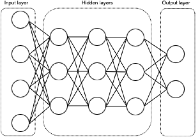
The multilayer Perceptron (MLP) is the simplest type of neural network and is a learning algorithm inspired by the function of neurons in the human brain. MLP is a feed-forward neural network that maps sets of inputs to sets of corresponding outputs. It comprises multiple layers of nodes in a directed graph, where each layer is fully connected to the next layer. In an MLP, there are at least three layers: an input layer, an output layer, and one or more hidden layers. Having more than one hidden layer provides more leverage, effectively allowing the MLP to learn more complex functions. The input layer of the MLP is called so because it receives the input vectors. These vectors are passed to the hidden layers, where they are further processed before being finally passed to the output layer. Between every layer is an activation function, which determines the activation of a node and allows the learning algorithm to learn non-linear characteristics. A simple example of an MLP is illustrated in Fig. 1. The operation of an MLP with \(L\) layers can be summarized in Eq. (2) as follows:

where \(a^{(0)}\) is the input \(x\), \(a^{(L)}\) is the output \(y\), \(W^{(l)}\) and \(b^{(l)}\) are the weights and biases for layer \(l\), and \(\sigma\) is the activation function applied element-wise.

Convolutional Neural Network (CNN)

Convolutional Neural Networks (CNNs) are a type of neural network designed for processing data with a grid-like topology, such as images. They use 2-dimensional convolutions and are inspired by the biological processes of the human visual cortex. Similar to MLPs, CNNs have multiple layers, each consisting of neurons. They commonly consist of three types of layers: convolutional layers, pooling layers, and fully connected layers. The convolutional layers perform computations by applying a set of filters (or kernels) to the input, producing feature maps that capture various aspects of the input data. The pooling layers perform a downsampling operation along the spatial dimensions (width and height) to reduce computational demands and control overfitting. The fully connected layers are similar to those in MLPs, where each neuron is connected to every neuron in the previous layer, computing the hidden activations and the class scores for classification tasks. Overall, CNNs leverage the hierarchical pattern in data to build complex models for image recognition and other tasks involving grid-like data. A simple example of a CNN is illustrated in Fig. 2. The operation of a CNN with \(L\) layers can be summarized in Eq. (3) as follows:

where \(a^{(0)}\) is the input \(x\), \(a^{(L)}\) is the output \(y\), \(W^{(l)}\) and \(b^{(l)}\) are the filters (or kernels) and biases for layer \(l\), and \(\sigma\) is the activation function applied element-wise. The function \(\text {Conv}(W^{(l)}, a^{(l-1)})\) denotes the convolution operation.

SPECK

SPECK is an ARX lightweight block cipher proposed by the US National Security Agency (NSA) in 2013. The increased use and deployment of portable intelligent devices motivated the development of SPECK. SPECK was specifically designed for limited resource devices and comes in various block and key sizes. The SPECK cipher is tailored for remarkable performance in software implementations, ensuring that the ROM size of a device does not impede its fast implementation. While SPECK can also be used in hardware implementations, the SIMON cipher has been specifically designed for this purpose.

The flexibility in the design of SPECK is the reason it has ten different implementations. To elaborate, SPECK typically encrypts a block of \(2n\) bits, where \(n\), the word size, can take values of 16, 24, 32, 48, and 64 bits. The key sizes for SPECK vary depending on the block size and can be \(2n\), \(3n\), or \(4n\) bits. Therefore, the SPECK cipher is denoted as SPECK2n/nm, where the block size is 2n and the key size is nm. The following Table 3 provides details about the ten variants of SPECK, including their parameters where \(\varvec{\alpha }\) is the circular right shift amount, \(\varvec{\beta }\) is the circular left shift amount and \(\varvec{T}\) is the number of rounds.

This flexibility in key sizes allows SPECK to be adapted for different levels of security and performance requirements. Based on the combination of the block size and key size, the number of encryption rounds varies from 22 to 34.

In this work, we focus on applying our proposed framework to the SPECK-32/64 block cipher, which we also refer to as SPECK. An encryption round of the SPECK cipher involves a series of bitwise operations to transform the plaintext. We note that our implementation uses little-endian representation. The round function begins by splitting the plaintext of size \(2n\) into two parts, right word, \({X^1}\) and left word, \({X^0}\), each of size \(n\). Each round then proceeds with these two \(n\)-bit words. The word \({X^1}\) is circularly right-shifted by 7 bits. The shifted \({X^1}\) is then added to \({X^0}\) modulo \(2^n\), and this forms the modular addition operation. Finally, the round key is XORed to this result. On the other hand, for the right word, the \({X^0}\) is circularly left-shifted by 2 bits. Next, an XOR operation is performed between \({X^0}\) and the modified \({X^1}\), and the roles of \({X^1}\) and \({X^0}\) are swapped for the next round. For SPECK-32/64, this round function is applied a total of 22 times. The round function operations are denoted as a set of equations for the SPECK cipher, representing the operations on the left \({X^1}_{i}\) and right \({X^0}_{i}\) of the block during an encryption round as follows:

where \({X^1}_{i}\) and \({X^0}_{i}\) are the left and right \(n\)-bit words at round \(i\), \({X^1}_{i+1}\) and \({X^0}_{i+1}\) are the left and right \(n\)-bit words at round \(i+1\), \(\ggg 7\) represents a circular right shift by 7 bits, \(\lll 2\) represents a circular left shift by 2 bits, \(k_i\) is the round key for round \(i\), \(\oplus\) denotes the XOR operation. The Fig. 3 further illustrates a round function in SPECK. Each operation in the SPECK round function emits power side-channel leakage, as both bit shifting and modular addition consume power. In particular, the modular addition and XOR operations introduce nonlinearity and the secret key, respectively, in the leakage model, which can be exploited by side-channel adversaries²⁴.

Additionally, every round of the encryption requires a round key which is derived from the secret key. For SPECK-32/64, the 64-bit secret key is initially divided into four 16-bit words, denoted as:

where \(k_0\) is used as the first round key. The key schedule then iteratively generates 22 round keys (\(k_0, k_1, …, k_{21}\)) using the following:

where \(k_0\), the first word of the master key, is the first round key. The term \(l_i\) refers to the \(i\)-th 16-bit word of the master key, while \(l_{i+m-1}\) is the newly derived key word added to the key schedule. The notation \(\ggg n\) represents a circular right shift by \(n\) bits; for instance, \(k_i \ggg 7\) shifts the bits of \(k_i\) seven positions to the right, with overflowed bits wrapped to the left. The operator \(+\) denotes modular addition over \(2^{16}\), limiting the result to 16 bits. The symbol \(\oplus\) represents the bitwise XOR operation. The variable \(i\) is the round index, ranging from \(0\) to \(T-2\), where \(T\) is the total number of rounds. Lastly, \(k_i\) and \(k_{i+1}\) represent the current and next round keys, respectively.

For this research, we considered the SPECK-32/64 version, which has a 32-bit block size and a 64-bit key. Our side-channel analysis focuses on the first four rounds of the encryption function, ensuring that all the words of the secret key are involved. From Eq. (6), the least significant word or pair of bytes of the secret key, \(k_0\), directly maps to the first round key, \(r_0\). However, in subsequent rounds, the master key bytes do not map directly to the round keys. Instead, we compute \(l_{i+m-1}\), which is then used to derive the next round key, \(k_{i+1}\). Consequently, the computed round keys are iteratively used in the encryption process for each round.

In our side-channel analysis experiment, we can attack round 0 and directly recover the round key, \(k_0\), which corresponds to the last two bytes of the 64-bit secret key. For the remaining three key bytes, we extend our attack to rounds 1, 2, and 3 to recover the corresponding round keys \(k_1, k_2, k_3\). These round keys are functions of the secret key bytes as follows:

Since round keys, \(k_1, k_2, k_3\) will be known from our deep learning profiling attack, we can sequentially recover the missing key bytes, \(l_0, l_1, l_2\) as follows:

Thus, by recovering \(k_0, k_1, k_2,\) and \(k_3\) through side-channel analysis, we can fully reconstruct all the secret bytes of the 64-bit secret key. We also note that this combination of round keys are needed to fully reconstruct the 64-bit secret key. In general, a combination of the attack on four rounds is needed in order to recover the secret key.

Furthermore, in this work we have considered both the unprotected and protected SPECK-32/64 implementations, which will be described as follows:

Unprotected implementation

An unprotected implementation of the SPECK-32/64 block cipher is a straightforward implementation of the algorithm without any countermeasures against side-channel attacks, such as power analysis or timing attacks. In such an implementation, the cipher’s operations are typically optimized for performance, resulting in faster execution but potentially exposing sensitive data during intermediate steps. For example, power consumption during encryption may reveal patterns that can be exploited to recover secret keys or other sensitive data. While unprotected implementations are efficient and suitable for scenarios where side-channel attacks are not a primary concern, they are vulnerable to a wide range of attacks in environments where security is paramount, such as in embedded systems or cryptographic hardware devices. Therefore, unprotected implementations should only be considered in low-risk situations where speed is prioritized over security. Figure 3 is an unprotected implementation.

Protected implementation

A protected implementation of the SPECK-32/64 block cipher focuses on enhancing its security against side-channel attacks, such as power analysis or timing attacks, which may reveal sensitive information during cryptographic operations. To achieve this, several countermeasures can be employed, including the use of constant-time algorithms to eliminate timing variations, masking techniques to obfuscate intermediate values, and randomization to avoid predictable execution paths. In this approach, the algorithm’s round operations and key schedule must be carefully designed to ensure that no leakage occurs at any stage, and that variations in power consumption or execution time are minimized, regardless of the cryptographic input. By incorporating these protective measures, the SPECK-32/64 implementation can be safeguarded against common side-channel threats, providing a robust solution for secure encryption in embedded systems. The Fig. 4 illustrates a protected implementation utilizing a masking technique.

The masking process begins with the generation of two random masks, which are used to mask the two words derived from the plaintext. The “B2A” and “A2B” modules, representing Boolean-to-Arithmetic and Arithmetic-to-Boolean conversions, respectively, are integrated into the round function. Additionally, masking is applied to the round key and the resulting two words at the end of the round function, ultimately yielding the original unmasked values of \(x_{i+1}\) and \(y_{i+1}\).

Ensembles

Ensemble learning aggregates predictions from multiple models, or “learners,” to improve accuracy and robustness. By combining the strengths of different models, ensemble methods reduce the likelihood of overfitting, as each learner captures distinct aspects of the underlying training data. As a result, ensemble models often outperform individual models in terms of generalization and predictive performance. This approach is widely used in techniques like Random Forest, a classic example of ensemble learning in machine learning, and has also been successfully applied in deep learning. Ensemble learning can take several forms, including bagging (e.g., Bootstrap Aggregation), which trains multiple models on different subsets of the data to reduce variance and improve stability; boosting (e.g., AdaBoost, XGBoost), which sequentially trains models where each new model focuses on the errors of the previous ones to reduce bias; and stacking, where the predictions of multiple base models are combined using a meta-learner to enhance overall predictive performance.

Furthermore, notable works in SCA have proposed ensemble deep learning-based profiling attacks, demonstrating successful attacks on AES and ASCON ciphers. These studies employed either random search or genetic algorithm-based search to generate fifty different models from which the ensembles are formed^38,39,40,41. Similarly, our proposed DL-SCA ensemble profiling methodology leverages random search to generate fifty different models. The novelty of our work lies in being the first to apply this technique to the SPECK cipher.