

Comparison of Res_BP, TCN_BP, and MLP_BP
Tables 3 and 4 summarize the performance of all models for DBP and SBP when trained on datasets without calibration data and with increasing numbers of subject-specific calibration measurements. For this comparison, we trained and evaluated the models with Pulse_Vital.
Across all architectures, SBP prediction is consistently more challenging than DBP prediction, a trend observed in prior work9,10,14,15,16,18,19,20.
Introducing as few as three calibration measurements results in a substantial improvement in performance, as evidenced by higher Pearson correlation coefficients and lower SDs. However, further increases in the number of calibration measurements yield diminishing returns, with performance approaching a plateau (see Fig. 4).

Pearson correlation coefficient and SDs over different numbers of calibrations
Despite these gains, none of the models meet the AAMI criterion for SBP estimation (SD < 8 mmHg), even when calibration data are included. For DBP estimation, both Res_BP and TCN_BP already meet the AAMI standard after three calibration measurements, whereas the MLP_BP model fails to satisfy this criterion under all calibration conditions.
Regarding model architecture, all pairwise comparisons remained statistically significant after correction for multiple comparisons (all p < 0.05). TCN_BP and Res_BP demonstrated comparable performance, with statistically significant yet practically negligible differences in MAE and only small effect sizes (r < 0.15). For example, in the three-calibration setting, the comparison between TCN_BP and Res_BP yielded
$$ \begin{aligned} & {\text{DBP}}:\Delta {\text{MAE}} = 0.0{6}\;{\text{mmHg}},\;{95}\% \;{\text{CI }}\left[ { – 0.0{6}, \, 0.{18}} \right],r = 0.0{1}; \\ & {\text{SBP}}:\Delta {\text{MAE}} = 0.0{8}\;{\text{mmHg}},\;{95}\% \;{\text{CI }}\left[ { – 0.{11}, \, 0.{26}} \right],r = 0.0{2}. \\ \end{aligned} $$
In contrast, both TCN_BP and Res_BP substantially outperformed MLP_BP in all calibration conditions, with effect sizes ranging from r = 0.14 to 0.45. Exemplarily, in the three-calibration setting, the comparison between Res_BP and MLP_BP showed
$$ \begin{aligned} & {\text{DBP}}:\Delta {\text{MAE}} = – {1}.{76}\;{\text{mmHg}},\;{95}\% \;{\text{CI}}\;\left[ { – {1}.{99},\; – {1}.{55}} \right],r = \, 0.{42}; \\ & {\text{SBP}}:\Delta {\text{MAE}} = – {2}.{66}\;{\text{mmHg}},\;{95}\% \;{\text{CI}}\;\left[ { – {3}.0{5},\; – {2}.{28}} \right],r = \, 0.{36}. \\ \end{aligned} $$
Full results are reported in Supplementary Data.
Comparison of datasets based on MIMIC or VitalDB
In this section, we retrain the models on the Pulse_MIMIC dataset (based on MIMIC-III28) set using either no calibration or three calibration measurements, aiming to determine whether potential waveform asynchronicity in the dataset leads to performance degradation (Table 5).
Across nearly all the experiments, the models trained on the Pulse_Vital dataset (based on VitalDB30) consistently outperformed those trained on the Pulse_MIMIC dataset, except for MLP_BP (0 cal). We attribute this performance disparity to a limitation previously reported in the literature27,29, namely the presence of variable inter-signal delays among the PPG, ABP, and ECG waveforms in the MIMIC-III database. Such temporal misalignment may compromise accurate signal synchronization and thereby reduce the reliability of derived scalar features, particularly PAT.
To further examine this issue, we computed the PAT at all corresponding fiducial points between the PPG and ABP signals for both the Pulse_Vital and Pulse_MIMIC datasets (Fig. 5). When PAT was derived from PPG signals, the strongest correlations with systolic blood pressure (SBP) were observed for the PATs and PATic features, with consistently higher correlation coefficients for PP across all fiducial points. These associations were more pronounced in the Pulse_Vital dataset than in the Pulse_MIMIC dataset, as indicated by slightly stronger negative correlation coefficients and lower p-values. In contrast, when PAT was derived from ABP signals, the inter dataset discrepancy was substantially reduced. ABP-derived PAT demonstrated stronger, more statistically significant correlations and lower variability.

Pearson correlation coefficients for SBP (A) and PP (B), and corresponding p-values for SBP (C) and PP (D), evaluated on the Pulse_MIMIC and Pulse_Vital datasets via PPG or ABP signals.
To put our calculated correlations into perspective, PAT-SBP correlations have been reported to range from (− 0.37, − 0.54)33,34,35,36 to < − 0.811. Ranges vary depending on the methods used to detect the PAT, the datasets used, or the condition/task of the subjects. Additionally, in the abovementioned works, the correlation between PAT-SBP is usually greater than that between PAT-DBP, and this is also the case for our subsets (see Supplementary Data). The PAT-PP correlations were even greater (with lower p-values) than the PAT-SBP correlations were. To utilize that, we used the PP as an auxiliary prediction head in all our models, as described above in the Methods section.
We also observed that the correlations varied depending on the method used to calculate the PAT (foot vs slope vs intersect vs peak), with the PATp performing worse and PATic and PATs best in the Pulse_Vital set, aligning with other reported observations11,35. One possible reason for this finding11,31 is that at any point in the arterial tree, the pressure wave can be considered a summation of forward- and backward-traveling waves, which affects the peak of the PPG signal most.
The observed performance improvement can be largely attributed to the guaranteed temporal synchronization of the PPG, ABP, and ECG channels in VitalDB30, which enables more precise estimation of PAT. In contrast, the MIMIC-III dataset28 likely contains non-constant inter-channel delays that reduce the reliability of PAT-derived features. Although a fixed temporal offset could, in principle, be learned and compensated for by the model, time-varying delays introduce irreducible noise that cannot be consistently corrected, thereby degrading performance.
It is also important to consider differences in patient populations between the two datasets. VitalDB30 comprises surgical patients, whereas MIMIC-III28 includes ICU patients. The lower PAT–SBP correlation observed in the Pulse_MIMIC subset may therefore also reflect differences in physiological state and medication exposure, as ICU patients often exhibit greater hemodynamic instability and pharmacological intervention, both of which can alter vascular tone and pulse wave propagation characteristics.
Influence of auxiliary PP head on DBP and SBP prediction
In the previous section, we observed that PP showed an even stronger correlation with PAT than SBP. Since PATf, PATs, PATp, and PATic were included in the input feature vector, we hypothesized that incorporating PP labels as an auxiliary prediction task could further improve the prediction accuracy of DBP and SBP.
To evaluate this hypothesis, we compared the MAE and Pearson correlation coefficients for DBP and SBP predictions from models trained with and without the auxiliary PP prediction head, with no calibration and three calibrations (Fig. 6). For clarity, only SBP results are presented in this section, as SBP prediction represents the more challenging task. The corresponding DBP metrics are provided in Supplementary Data.

Comparison of Model Performances for SBP Prediction with and without (no PP) auxiliary PP head
Overall, models with and without the auxiliary PP head performed comparably. For instance, comparing Res_BP with Res_BP (no PP) under the no-calibration condition yielded only a marginal difference (ΔMAE = 0.12 mmHg, 95% CI [− 0.09, 0.34], r = 0.028). Slightly larger differences were observed under the three-calibration condition (ΔMAE = − 0.34 mmHg, 95% CI [− 0.49, − 0.18], r = 0.114), though the overall effect size remained small. Similarly, comparing TCN_BP with TCN_BP (no PP) revealed negligible differences (ΔMAE = 0.03 mmHg, 95% CI [− 0.15, 0.21], r = 0.001).
One plausible explanation for the limited impact of the auxiliary PP head is that PP is not an independent physiological quantity but is directly derived from SBP and DBP (PP = SBP − DBP). Since the network already jointly predicts SBP and DBP from a shared latent representation, the auxiliary PP task likely provides only a marginal additional supervisory signal during optimization. As a result, the auxiliary task may have acted as a redundant constraint rather than introducing complementary physiological information capable of substantially improving blood pressure estimation performance.
Comparison with other models
Some studies have reported high predictive performance, with correlation coefficients ranging from 0.966 to 0.977 for systolic blood pressure (SBP) and from 0.947 to 0.964 for diastolic blood pressure (DBP), along with standard deviations (SD) of 3.35 mmHg and 2.44 mmHg17,37, passing the AAMI test and receiving a BHS Grade A for DBP and SBP. Both models were trained on MIMIC-based datasets.
Notably, the AAMI test requires the standard deviation of the mean error (ME), not of the mean absolute error (MAE), which was calculated in the above-mentioned studies. Usually, the SD of the ME is bigger than that of the MAE because neglecting the sign of the error reduces the variance17,37.
In this work, we wanted to investigate the extent to which data leakage may influence evaluation metrics. Therefore, we re-examined the models described in17,37 because they were well documented. In addition, we added reduced-capacity variants of these models by reducing the layer depth and number of filters in the DeepBP37 model (denoted as DeepBP small), and the hidden layer width and depth in the MLP OG17 model (denoted as MLP OG small). These reduced-capacity variants were included to assess how model capacity affects data leakage and evaluation performance.
In the first experiment, the models were retrained using the MIMIC-BP dataset, which applies a subject-wise data split while maintaining an equal number of samples per subject. Furthermore, instead of extracting a single 8.5 s window from each segment, we generated multiple non-overlapping 2 s windows per segment, a common strategy for increasing dataset size. The MIMIC-BP dataset was selected over Pulse_MIMIC because its 30 s segments, compared with the 10 s segments in Pulse_MIMIC, allowed approximately three times as many samples to be extracted from each segment. This characteristic is particularly relevant for investigating potential data leakage effects. When multiple short windows are generated from the same underlying physiological segment, the resulting samples are inherently highly correlated, despite being non-overlapping. Consequently, if leakage exists between training and test partitions, the larger number of derived windows in MIMIC-BP is expected to amplify its impact on evaluation metrics. In the following section, we report the metrics for SBP, as it’s generally more challenging to predict than DBP.
Using our dataset and the subject-wise data split in our training pipeline, we were unable to reproduce the reported high correlations and low MAEs. In fact, our models showed lower errors and higher Pearson correlations. Overall, the MEs and SDs were in the range of previously reported models, ResNet15226 and PPG2ABP v238, where a subject-wise data split was enforced (Table 6).
In the second experiment, we repeated the training process, this time allowing segment data from each subject to appear in the training, validation, and test sets.
In this setting, we were able to reproduce the overall performance trends reported in prior works (Table 7), however, our Res_BP, TCN_BP, and MLP_BP models consistently underperformed the larger reference models. Assuming that data leakage contributes substantially to these results, a plausible contributing factor to the observed discrepancies is model capacity. DeepBP37 and the MLP model in17 contain approximately \(2.1\times {10}^{6}\) and \(5.9\times {10}^{7}\) total parameters (7.84 MB and 224 MB), respectively. A performance degradation was observed in the reduced-capacity variants DeepBP small and MLP OG small, which contain approximately \(1.3\times {10}^{5}\) and \(1.1\times {10}^{6}\) total parameters (0.50 MB and 4.03 MB), respectively. In contrast, our models without calibration processing comprise only \(1.0\times {10}^{3}\) to \(2.3\times {10}^{4}\) parameters (3.9 kB to 90.3 kB).
Under data leakage conditions, the substantially larger DeepBP37 and MLP OG17 models likely benefited from their high representational capacity, enabling them to memorize subject-specific patterns rather than learn generalizable physiological relationships. This may also explain why MLP OG17, which is approximately 29 times larger than the second-largest model DeepBP37, achieved the best performance. Furthermore, progressively reducing the model capacity resulted in increased ME, SD, MAE, and STD values, suggesting that the smaller models approached their capacity limits and were therefore less capable of memorizing subject-specific information. This interpretation is further supported by the comparatively large effect sizes observed under data leakage conditions (r = 0.44 – 0.61), indicating substantial statistical differences between the large-capacity models and their reduced-capacity variants (Table 8).
In contrast, when a strict subject-wise data split was applied, the larger models, DeepBP37 and MLP OG17, did not outperform their reduced-capacity counterparts, DeepBP small and MLP OG small. Although all pairwise comparisons remained statistically significant after correction for multiple comparisons (all p < 0.05), the observed differences in mean MAE and effect sizes were small (r = 0.03 – 0.12), indicating only minor practical differences between model variants despite statistical significance (Table 8). These findings suggest that, in the absence of data leakage, the larger capacities of the original models did not improve the performance of the reduced-capacity variants.
Interestingly, under the subject-wise data split condition, the largest performance difference was observed between the comparatively small TCN_BP model (90.3 kB) and the substantially larger MLP OG17 model (224 MB). Specifically, TCN_BP achieved a lower mean MAE difference (ΔMAE = − 0.83 mmHg) and the largest observed effect size in this setting (r = 0.12), indicating a slight performance advantage over MLP OG17. This suggests that the reduced capacity of the smaller model may have been beneficial, as it constrained the model to learn more generalizable representations rather than overfitting to subject-specific characteristics. This interpretation is further supported by slightly lower SD, MAE, and STD values, as well as higher Pearson correlation coefficients observed for the smaller models. However, given the small effect size, these findings should be interpreted with caution and do not imply that the smaller models consistently generalize better than their high-capacity counterparts.
A commonly used data augmentation strategy is to divide each segment into multiple shorter windows. While this approach can effectively increase the number of training samples, it requires careful handling to avoid data leakage. In datasets such as MIMIC-BP, where individual segments span 30 s, both the PPG waveform and the associated SBP and DBP values exhibit limited variability within a single segment, which could further amplify the memorization effect.
For demonstration, we partitioned each 30 s MIMIC-BP segment from one subject into multiple non-overlapping 2 s windows and overlaid the corresponding PPG and ABP waveforms (see Fig. 7, windows A and B). SBP and DBP were computed as the maximum and minimum values within each 2 s window, respectively. The within-segment standard deviations were only 0.42 mmHg for DBP and 0.76 mmHg for SBP, indicating very limited blood pressure variability over the full 30 s interval and a high degree of similarity between the PPG and ABP signals.

Overlayed 2 s PPG (A) and ABP (B) waves of one 30 s segment of subject 132. (C, D) displays the resulting DBP and SBP of all segments across one subject
Consequently, if multiple windows from the same segment are distributed across both training and test sets, a model may achieve artificially high accuracy by memorizing waveform–blood pressure pairs rather than learning physiologically meaningful relationships.
Nonetheless, the observed performance differences cannot be attributed solely to data leakage, as the present study also differs from17,37 in several other aspects, including the training and testing datasets, the applied filtering and preprocessing pipelines, the chosen training hyperparameters, and the choice of input data, such as signal length and scalar input features.
One could argue that the calibration approach used in this work also constitutes a form of data leakage. Here, the first three to nine measurements from separate segments were used for calibration. This stands in contrast to prior works, where data leakage is likely more pronounced: in those studies, all available samples were randomly shuffled into training and test sets, with samples from the same segment appearing in both17,23,37.
Using a few segments from the same subject—for example, reserving the first three to nine segments for calibration as well as using only one sample per segment—is substantially less prone to overfitting and memorization. As illustrated in Fig. 7C–D, the DBP and SBP values for a single subject vary noticeably across the 30 available segments (Segment DBP Std: 8.61 mmHg; Segment SBP Std: 14.50 mmHg). In this setting, the model cannot rely on simple memorization. Instead, it must learn patterns associated with blood pressure variation across time. When calibration data are available, the model additionally learns subject-specific offsets (e.g., associations between PAT and DBP, SBP), capturing how blood pressure deviates from an individualized baseline rather than memorizing absolute values.
Comparison of the PPG data with the ABP data (Pulse_Vital)
To assess how signal fidelity and derived temporal features (e.g., PAT) affect prediction performance, we replaced the PPG waveform with the ABP waveform as the model input, using the Pulse_Vital set. To prevent data leakage and ensure subject-independent learning, the ABP signals were z-normalized at the individual subject level prior to model training.
The motivation for using ABP data lies in its superior representation of cardiovascular physiology. Unlike PPG, which provides an indirect optical measurement of peripheral blood volume changes and is highly sensitive to external factors such as sensor placement, contact pressure, skin properties, and motion artifacts, ABP directly measures intra-arterial pressure dynamics. As a result, the ABP waveform preserves critical morphological characteristics—including systolic upstroke, diastolic decay, and the dicrotic notch—that are closely linked to arterial compliance, vascular resistance, and wave reflection phenomena. These features are either distorted or partially lost in PPG recordings, limiting their physiological expressiveness for blood pressure estimation (compare PPG and ABP in Fig. 7A,B).
In our experiment, all models benefit from using ABP both as the input signal and for feature extraction (compare dashed PPG curves versus solid ABP curves in Fig. 8). The most pronounced improvements were observed in systolic blood pressure (SBP) prediction for models without calibration data, with Pearson correlation coefficients increasing by 58–62%. Notably, the TCN_BP and Res_BP configurations met the AAMI criteria for both DBP and SBP estimation when at least three calibration measurements were included. These models achieved Grade A performance for DBP and Grade A for SBP with Res_BP and Grade B for SBP with TCN_BP. In contrast, none of the PPG-based models satisfied the AAMI requirements for SBP estimation.

Model performances when the PPG or ABP waves are used as inputs. (A, B) displays the Pearson correlation. (C, D) SD according to AAMI
The statistical model comparison of Res_BP vs TCN_BP vs MLP_BP, after correction for multiple comparisons (all p < 0.05), revealed statistical significance, yet with small ΔMAE and effect sizes for TCN_BP vs Res_BP, indicating that these two models performed comparably, while Res_BP performed significantly better than MLP_BP, indicated by large ΔMAE and effect size. Exemplary for the condition with three calibrations:
$$ \begin{aligned} & {\text{TCN}}\_{\text{BP vs Res}}\_{\text{BP}}: \\ & {\text{DBP}}:\Delta {\text{MAE}} = 0.{4}\;{\text{mmHg}},\;{95}\% \;{\text{CI }}\left[ {0.{28}, \, 0.{5}0} \right],r = \, 0.{19}; \\ & {\text{SBP}}:\Delta {\text{MAE}} = 0.{31}\;{\text{mmHg}},\;{95}\% \;{\text{CI }}\left[ {0.{14}, \, 0.{48}} \right],r = \, 0.0{7}. \\ \end{aligned} $$
$$ \begin{aligned} & {\text{Res}}\_{\text{BP vs MLP}}\_{\text{BP}}: \\ & {\text{DBP}}\Delta {\text{MAE}} = – {3}.{36}\;{\text{mmHg}},\;{95}\% \;{\text{CI }}\left[ { – {3}.{66}, \, – {3}.0{7}} \right],r = \, 0.{59}; \\ & {\text{SBP}}:\Delta {\text{MAE}} = – {5}.{67}\;{\text{mmHg}},\;{95}\% \;{\text{CI }}\left[ { – {6}.{11}, \, – {5}.{23}} \right],r = \, 0.{66}. \\ \end{aligned} $$
A full overview of Model metrics and statistics across no, three, six, and nine calibrations for DBP and SBP is provided in the Supplementary Data.
Interestingly, a slight increase in SD was observed when the number of calibration measurements increased from three to six in the ABP setting (Fig. 8). Although the differences were small overall, this finding suggests that additional calibration measurements did not lead to a strictly monotonic improvement in performance in this dataset. Notably, the SD obtained with nine calibration measurements was again slightly lower than that observed with three calibrations, indicating a non-linear relationship between the number of calibration samples and model performance. One possible explanation is that subject-specific adjustment may already be adequately captured using a small number of calibration samples, while intermediate increases in calibration measurements could introduce additional variability related to physiological fluctuations or measurement noise. With a larger number of calibration samples, however, the effect of such variability may be partially compensated by averaging across more measurements. However, these interpretations remain speculative, as they were not explicitly tested in the present study. In addition, the observed pattern may be sensitive to the random seed used (seed 42). Further robustness analysis using multiple random seeds and repeated training runs would be necessary to assess the stability of this trend.
Finally, Res_BP and TCN_BP demonstrated larger performance improvements when using ABP waveform signals. MLP_BP model, which relied solely on scalar features such as PAT derived from ECG-to-PPG or -ABP, showed only minimal or no improvement. This suggests that although MLP_BP underperforms overall compared with Res_BP and TCN_BP, the scalar features used in this study (e.g., PAT) are less sensitive to temporal shifts when extracted from PPG or ABP signals.
The predictive performance of the Res_BP model, calibrated with three measurements, was assessed for diastolic blood pressure (DBP) and systolic blood pressure (SBP) via correlation and Bland–Altman analyses (Fig. 9). Density-colored scatterplots indicate that regions with higher sample density, corresponding to more frequently observed BP values, are predicted more accurately by the model.

Correlation and Bland–Altman plot of DBP and SBP for the best performing model, Res_BP with three calibration measurements. The rainbow color coding shows the amount of the data, with red indicating high amount of data and blue indicating low amount of data
Especially for SBP, higher values tend to exhibit larger prediction errors, with the model generally underestimating true SBP. This pattern has also been observed in previous studies, as summarized by7, who attributed it to an imbalance phenomenon in BP datasets, in which skewed distributions bias predictions toward central BP values. In Fig. 10, for example, the number of samples with SBP > 160 mmHg was substantially lower than that in lower ranges. No strategies to correct this imbalance were applied in this work.
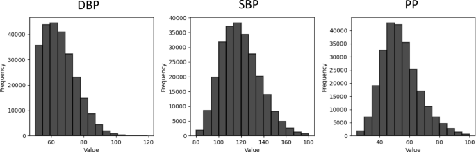
Histogram of DBP, SBP and PP in the Pulse_Vital Train Set
Overall, the findings demonstrate that the blood-flow representation captured by PPG does not adequately encode the pressure-related information required for reliable SBP prediction in the Res_BP and TCN_BP models, which jointly process waveform and scalar features. The larger performance improvements observed for SBP indicate that systolic pressure estimation is more sensitive to signal fidelity than DBP estimation. As illustrated in Fig. 7 (A vs B), the PPG waveform fails to reproduce key pressure wave characteristics, especially visible with the missing dicrotic notch.
In contrast, DBP could be estimated with acceptable accuracy from PPG signals when at least three calibration measurements were available. However, even the ABP-based models required a minimum of three calibration measurements to meet the AAMI performance criterion for DBP estimation.


