Classifying human vs. AI text with machine learning and explainable transformer models

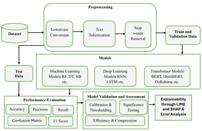
Performance metrics

In evaluating the performance of machine learning, Recurrent Deep Learning, and transformer-based models for classifying GPT-generated versus human-written text, a comprehensive suite of performance metrics was employed to ensure robustness and practical applicability. These metrics include the confusion matrix, accuracy, precision, recall, and F1 score, each offering critical insight into various aspects of model behavior. The confusion matrix is particularly valuable as it outlines the distribution of true positives (TP), false positives (FP), true negatives (TN), and false negatives (FN). This breakdown enables detailed analysis of misclassification trends i.e., distinguishing whether the model tends to misclassify human-written content as AI-generated or vice versa. Such insights are crucial for refining model behavior in real-world applications, where subtle linguistic cues can cause confusion between classes.

Accuracy, defined in Eq. (1), measures the proportion of correctly predicted instances out of all predictions. While it provides a general sense of performance, it can be misleading in the presence of class imbalance such as when the dataset contains more GPT-generated samples than human-written ones. Therefore, accuracy must be interpreted in conjunction with other metrics.

Precision shown in Eq. (2), evaluates the correctness of the model’s positive predictions. In the context of this task, high precision indicates that when the model predicts a text as GPT-generated, it is usually correct. This helps reduce false alarms, ensuring that naturally written human content is not mistakenly flagged as AI-generated.

Recall defined in Eq. (3), assesses the model’s ability to correctly identify all relevant instances of a class. A high recall means the model can effectively detect most GPT-generated content, minimizing the likelihood that such texts go unnoticed.

The F1 score presented in Eq. (4), provides a harmonic mean of precision and recall, serving as a balanced metric particularly useful when both false positives and false negatives are costly. For example, in content moderation or academic integrity settings, misclassifying human work as AI-generated (or vice versa) can have significant consequences. A high F1 score thus indicates the model’s strong overall ability to make accurate and reliable distinctions between the two text types.

Collectively, these metrics offer a well-rounded evaluation framework. They enable not only assessment but also iterative refinement of models, ensuring that the system accurately distinguishes between GPT-generated and human-written text with minimal risk of misclassification.

Experimental settings

All experiments were conducted using Kaggle’s cloud-based platform, which provides access to powerful computing resources including free GPUs. The environment supported Python 3 with libraries such as Scikit-learn, TensorFlow, Keras, PyTorch, and HuggingFace Transformers. The dataset was uploaded and processed directly within Kaggle Notebooks. Pre-trained embeddings (e.g., FastText) and transformer models (e.g., BERT, RoBERTa) were loaded from external sources or integrated via HuggingFace. Model training, evaluation, and visualization were performed end-to-end within this environment, ensuring a reproducible and scalable experimental setup.

In this study, various hyperparameters were carefully selected and tuned for machine learning, recurrent deep learning and transformer models to ensure optimal performance. Each model was fine-tuned using carefully selected hyperparameters to optimize performance. The detailed explanation regarding hyperparameters such as batch size, Optimizer, sequence length, dropout rate, learning rate, number of epochs etc., is provided in Table 4. some were varied according to models used.

Performance evaluation

To assess the effectiveness of various models in distinguishing between Human-Generated and GPT-Generated text, extensive experiments were conducted using traditional machine learning models, deep learning architectures, and state-of-the-art transformer-based models. The evaluation metrics included confusion matrix, Accuracy, Precision, Recall, and F1 Score.

Among classical algorithms shown in Table 5, RF consistently achieved higher accuracy across embeddings, with Word2Vec-based features yielding up to 0.788 accuracy. The performance of Logistic Regression was equally strong, especially with Word2Vec (0.783) and FastText (0.796), while SVM achieved competitive results with FastText (0.794). Naïve Bayes and Decision Tree models showed relatively lower performance, highlighting their limitations in capturing complex semantic patterns. Overall, the ML models achieved superior performance when integrated with FastText embeddings compared to Word2Vec and GloVe, highlighting FastText’s effectiveness in capturing contextual and subword-level information.

Recurrent Deep Learning approaches demonstrated (Table 6) notable improvements over traditional ML models. LSTM and GRU architectures, along with their bidirectional variants, consistently outperformed simple RNNs. The best performance was observed with BiLSTM (Seed = 123, Dim = 200) and BiGRU (Seed = 123, Dim = 200), achieving accuracies of 0.8457 and 0.8467, respectively. These models effectively captured sequential dependencies and contextual information, contributing to superior recall and F1-scores. While RNNs showed stable performance, their results were generally lower compared to LSTM and GRU families, confirming the importance of gated mechanisms in handling long-term dependencies.

In contrast, the performance of Transformer-based models shown in Table 7 demonstrates a significant superiority over both classical machine learning and recurrent deep learning baselines, underscoring their strong capability in capturing complex contextual representations. For example, BERT achieved the highest overall accuracy of 0.9637 with an epoch value of 3, with balanced precision, recall, and F1-scores, indicating strong generalization. RoBERTa, mBERT and DeRoBERTa also delivered competitive results, with accuracies of 0.9617, 0.9530 and 0.9480, respectively, while ALBERT maintained slightly lower but stable performance. The results demonstrate that transfer learning with pre-trained transformer architectures provides substantial improvements over traditional embeddings and models by leveraging large-scale contextual knowledge.

Additionally, the study reports the performance of transfer learning models with 95% confidence intervals (CIs) computed over three random seeds (7, 42, and 123) for all key metrics, and further assess statistical significance and calibration reliability. Table 8 summarizes the results at epoch 3, identified in Table 7 as the optimal convergence point for most models. RoBERTa achieved the highest accuracy (0.961 ± 0.004) and F1-score (0.962 ± 0.004), followed by XLM-RoBERTa and BERT, while DeBERTa attained the best recall (0.991 ± 0.007) at the expense of precision, indicating a recall–accuracy trade-off. Paired McNemar tests confirmed the statistical significance of differences between BERT and the top-performing models. Calibration analysis further validated reliability, with RoBERTa exhibiting the lowest Brier score (0.034 ± 0.003) and stable ECE values across models. In terms of efficiency, DistilBERT required the least GPU time (0.862 h), highlighting its resource-friendliness despite slightly lower accuracy.

Furthermore, to evaluate the generalization capacity of RoBERTa, its classification performance was compared across three dataset versions: the original, a 5–10% human-edited, and a 30–40% human-edited version. This experiment aimed to examine the model’s robustness and brittleness under varying levels of realistic human post-editing. The results (Table 9) indicate that RoBERTa maintained strong performance on both edited datasets. For the 5–10% human-edited data, accuracy (0.951 ± 0.014) and F1 score (0.953 ± 0.012) were close to the original dataset (0.961 ± 0.004 accuracy, 0.962 ± 0.004 F1), showing minimal degradation. However, at higher editing levels (30–40%), performance slightly decreased (0.9442 ± 0.0142 accuracy, 0.9466 ± 0.0128 F1), indicating modest sensitivity to extensive paraphrasing. Interestingly, recall remained consistently high (0.987–0.988 ± 0.003), reflecting the model’s stability to detect positive cases. Calibration metrics (Brier/ECE) exhibited negligible variation across datasets, suggesting that human text edits particularly at moderate levels had limited influence on the reliability of RoBERTa’s confidence estimates.

To assess the reliability of RoBERTa’s confidence estimates, temperature scaling was employed as a post-hoc calibration technique. The fitted temperature value was 1.476, which adjusted the model’s softmax outputs to better align predicted probabilities with actual outcomes. Before calibration, the Expected Calibration Error was approximately 0.4923, indicating substantial overconfidence. Temperature scaling effectively reduced miscalibration, improving the reliability of probability outputs. Figures 6 presents the reliability diagrams before and after calibration, respectively. The diagonal orange line represents perfect calibration, while deviations from this line reflect over- or under-confidence. As seen, calibration improves the model’s reliability across most confidence bins.

In addition, threshold tuning was performed to prioritize precision for high-stakes predictions. The optimal threshold achieving ≥ 90% precision was t = 0.957, resulting in precision = 0.963 and recall = 0.963. These adjustments enhance the interpretability and trustworthiness of the model’s outputs in practical applications.

To confirm whether observed performance differences between transformer models were statistically significant, McNemar’s test was conducted with Holm correction for multiple comparisons. The results (Table 10) revealed significant differences between all model pairs (p < 0.05). Specifically, XLM-RoBERTa vs. RoBERTa (p = 0.0195) and BERT vs. RoBERTa (p = 2.99 × 10⁻⁶) showed statistically reliable improvements in favor of RoBERTa. Although the effect sizes (Cohen’s g = 0.005–0.010) were small, they support the conclusion that RoBERTa’s performance advantages are consistent and not due to chance.

In addition to accuracy metrics, inference efficiency was assessed through latency and throughput measurements (Table 11). RoBERTa achieved a balanced trade-off between speed and accuracy, with an average latency of 0.2935s per prediction and throughput of 68.1 texts/sec. XLM-RoBERTa demonstrated the highest throughput (69.1 texts/sec), while BERT was comparatively slower (63.2 texts/sec). These findings indicate that RoBERTa offers an optimal balance of computational cost and predictive reliability.

To assess potential for model compression, a global unstructured pruning experiment (20%) was conducted on RoBERTa. The pruned model maintained similar predictive behavior on a small validation sample, demonstrating the feasibility of parameter reduction without significant accuracy loss. This aligns with sustainability-oriented objectives by reducing computational demands while preserving interpretability.

A fine-grained error analysis was performed to evaluate RoBERTa’s robustness across text length categories. Results presented in Table 12 indicate that performance remained consistently high across all bins, with perfect scores for very short, short, and long inputs (F1 = 1.000) and only a minor drop for medium-length samples (F1 = 0.952). This suggests that the model generalizes effectively across varying input complexities and message lengths.

Explanations results

To enhance model transparency, LIME and SHAP was applied to the RoBERTa model predictions. LIME explains individual predictions by perturbing input text and approximating the model’s decision boundary with a simpler, interpretable model. As shown in Fig. 7, words such as “honestly,” “never,” “corsetry,” and “intrigued” were highlighted as strong contributors toward the Human class. The color intensity represents each token’s influence on the classification, helping to understand which linguistic features RoBERTa used in making its decision.

Additionally, SHapley Additive Explanations provided a more theoretically grounded interpretation. SHAP assigns Shapley values to each token, indicating their positive or negative contributions to the output probability. In Fig. 8, red-colored tokens such as “intrigued” push the prediction toward the Human class, while blue tokens like “the rabbit hole” slightly pull it in the opposite direction. SHAP ensures that the contributions sum up to the predicted probability, offering a globally consistent and fair explanation of feature importance.

In the Fig. 9 focused on the LIME explanation shows that the model classified the input text as GPT with 100% probability, leaving no chance for Human. The highlighted words such as “and,” “are,” “of,” “to,” “without,” and “user” contributed most to the GPT prediction. These are mostly function words and connectors, which LIME suggests are strong signals of GPT-generated writing. In other words, the model associates GPT text with structured sentence flow and frequent use of linking terms, rather than with domain-specific keywords.

The SHAP explanation (Fig. 10) also predicted the text as GPT with a probability of 0.9980. Unlike LIME, SHAP distinguishes between words pushing the prediction towards Human (blue) and GPT (red). Terms such as “Spyware,” “designed,” and “collect” leaned towards Human classification, as they resemble natural human writing and technical terminology. However, words like “without” and “consent” strongly pushed the decision towards GPT, highlighting how formal connectors and rigid phrasing are characteristic of machine-generated text.

In short, LIME provides a quick and visually intuitive understanding of which words influence RoBERTa’s predictions, making it ideal for fast debugging and local interpretability. SHAP, on the other hand, offers a more precise and mathematically consistent explanation by fairly distributing contributions among all tokens. While LIME is computationally lighter and easier to implement, SHAP is preferred when a deeper, globally consistent interpretation is required, especially in research or high-stakes decision-making scenarios.

In addition to local explainability, which focuses on understanding individual predictions, global explainability provides a broader view of the model’s behavior across the entire dataset. As shown in the Permutation Feature Importance (PFI) plot (Fig. 11), the token “which” stands out with the highest importance score of 2.0, indicating it has the greatest impact on model predictions when perturbed. Other tokens such as “case-insensitive.”, “discern”, “complexity”, and “Paris.” have lower but consistent importance values of 1.0, suggesting they also contribute meaningfully to the model’s overall decision-making. The baseline accuracy of 0.975 further supports the model’s robustness. To ensure global stability, agreement metrics across multiple runs or random seeds can be incorporated, confirming that the importance rankings are not sensitive to small variations in training.