
Banana exports in India during 2020–2021 exceeded INR 616 crores. As the year progresses, the number of banana plants also increases, resulting in higher demand for the fruit. Therefore, the aim is to cultivate more banana plants that are disease-free. Several authors have focused on the early detection and prediction of banana leaf diseases, outlining six major steps in the process. Figure 7 depicts the process of predicting banana leaf diseases.
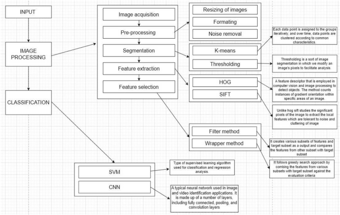
Processes involved in prediction2,3,13.
Image acquisition
Image acquisition is a crucial task that must be carried out before proceeding with any other processes. This phase involves capturing images with proper lighting, angle, and depth to ensure high resolution and quality. Capturing high-quality images ensures effective feature extraction in the subsequent phase. Additionally, it provides auto-exposure and auto-focus for image pre-processing1,16. After completing the image acquisition task, the next step is to preprocess the image by removing any noise present.
Pre-processing
The pre-processing phase receives input from the image acquisition phase and performs minor modifications before sending the image to the next phase. The modifications involved in the process include resizing and formatting of images (SVG/PNG), as well as noise removal. The focus of the noise removal process is to identify defects and achieve greater accuracy1,46. After completing pre-processing and noise removal, the image input is sent to the segmentation layer to select the significant components of the image, making the subsequent task much simpler1,3.
Segmentation layer
Segmentation receives input images from the pre-processing layer to select the shape and colour of the affected region, as well as the background color, among other factors29. This can be achieved using any of the following methods.
K-means clustering
This concept is implemented to identify the infected banana leaves by considering two distinct data points. The first data point corresponds to the highlighted portion, which is assumed to be the diseased section. The second data point corresponds to the dark portion, indicating the healthy portion47. The K-means clustering algorithm calculates the “centroids” of a set of N data points and computes the Euclidean distance. This process results in the formation of a cluster consisting of data points that are closer to a specific centroid. Once two distinct clusters are obtained from the data sets, the centroids of the clusters need to be recomputed. The process is then repeated by computing the Euclidean distance between all the data points and the new centroid. This iterative process of forming clusters continues until the centroids no longer undergo significant changes. The initial centroids are selected as K-objects, and nearby objects are assigned to the closest centroids26,48.
Thresholding
This methodology transforms the provided image, which may be in color or grayscale, into a simplified binary image through the suitable manipulation of pixels. By means of this conversion, the original image is partitioned into two distinct regions, specifically objects and background. If the intensity distribution of pixels in the image exhibits sufficient disparity, a single threshold value is sufficient for the entire image, known as a global threshold. In the context of a banana leaf image, in which f(x, y) represents a pixel containing a light object (the diseased portion) against a dark background, an appropriate threshold value, denoted as T, is diligently chosen to effectively discriminate between a diseased leaf and a healthy one by segmenting the intensity of the pixel. Dark portions correspond to healthier regions, while light portions indicate the presence of a diseased leaf26. The subsequent step involves the extraction of features, which is accomplished through the classification of all the aforementioned features.
$${\text{Let}}\,{\text{X}}\left( {{\text{i}},{\text{j}}} \right)\,{\text{be}}\,{\text{an}}\,{\text{image}}\,{\text{X(i,j) = }}\left\{ {\begin{array}{*{20}l} {0,} \hfill & {\text{p(i,j) < T}} \hfill \\ {1,} \hfill & {{\text{p(i,j)}} \ge {\text{T}}} \hfill \\ \end{array} } \right.$$
where p(i,j) is the pixel value at position (i,j), and T being the threshold value26.
Feature extraction layer
After completing the segmentation process, the feature extraction phase studies the number of pixels in the image and captures significant information by identifying similar feature sets and distinguishing dissimilar ones. This process is also used to differentiate between healthy and affected banana leaf plants. To study the number of pixels in an image and extract the feature vector, follow the process outlined in49.
HOG feature (histogram of oriented gradients)
Histogram of Oriented Gradients (HOG) is a method used in image processing and computer vision for object detection4. It calculates features by identifying healthy regions using intensity gradients to distinguish affected regions. This approach operates on cells and is not affected by image transformations. Other methods, such as Hu moments, Haralick texture, and color histograms, may also be used in the process.
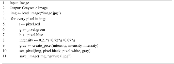
Hu moments are utilized to extract the outline of an object in the provided image. This is accomplished by converting the given image of a banana leaf from RGB to grayscale to highlight the outline of the leaf. Hu moments are then applied to characterize the pixels of the banana leaf in the image1,2.
Heralick texture features are functions of the Normalized Gray Level Co-occurrence Matrix (GLCM), which counts the co-occurrence of neighbouring gray levels in the given image. The GLCM is a square matrix that represents different aspects of the gray-level distribution in the Region of Interest (RoI). In predicting banana leaf disease, healthy and affected regions exhibit different textures. The process differentiates between the textures of healthy and affected regions in the banana leaf by utilising the adjacency matrix or GLCM matrix1,49,50.
The different texture features are given by31
$${\text{Range }} = { }\left[ {\left( {{\text{size}}\left( {{\text{GLCM}},{ }1} \right){ } – { }1} \right)} \right]^{2}$$
(1)
$${\text{Contrast }} = \mathop \sum \limits_{i,j = 0}^{N – 1} {\text{p}}\left( {{\text{i}},{\text{j}}} \right)\left| {{\text{i}} – {\text{j}}} \right|^{2}$$
(2)
(Where p(i,j) = pixel of the image)
$$\text{Correlation }=\sum_{i,j=0}^{N-1}\text{p}\left(\text{i},\text{j}\right)\left|\frac{\left(\text{i}-{\mu }_{i}\right)\left(j-{\mu }_{j}\right)}{\sqrt{{\sigma }_{i}^{2}{\sigma }_{j}^{2}}}\right|$$
(3)
$$\text{Energy}=\sum_{i,j=0}^{N-1}{p(i,j)}^{2}$$
(4)
$$\text{Homogeneity}={\sum }_{i,j=0}^{N-1}\frac{p\left(i,j\right)}{1+{\left(i-j\right)}^{2}}$$
(5)
$$\text{Entropy}=\sum p{\text{log}}_{2}p$$
(7)
(p = normalized histogram count).
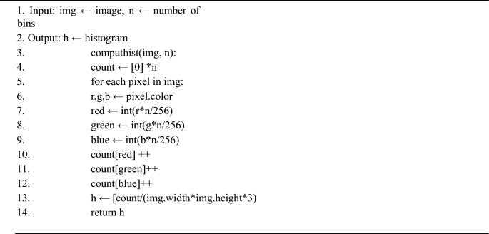
The colour histogram technique is widely used to extract image colour features. Typically, RGB or HCV colour spaces are used, but for multispectral images, an N-dimensional colour histogram is used. However, due to the difficulty in representing N-dimensional histograms, RGB is often used by narrowing down the banana leaf into 256 colours to achieve maximum accuracy. This process results in the creation of four bins with varying intensities and intervals. The respective intensities of each bin are listed in Table 3.
Finally calculate the pixel count in each bin to draw the color histogram for the banana leaf1,2.
Scale invariant feature transform (SIFT)
The Scale Invariant Feature Transform (SIFT) algorithm is designed to detect and describe local features, also known as ‘key points’, in an image. The SIFT process includes several phases: Space Generation, Difference of Gaussians (DoG), Key Point Detection, and Feature Description. Unlike the HOG method, the SIFT method only studies the significant pixels of the image to extract local features, making it more effective. This method identifies the important key points of both the affected and unaffected regions of the leaf. The key points are then grouped using k-means clustering or LS function. Various feature vectors are calculated for different clusters. The direction and magnitude of these key points are determined using neighboring pixels, and each key point is represented as a 128-dimensional feature vector22,32.
$${\text{D }} = \, \left\{ {\left( {{\text{xi}},{\text{ yi}}} \right)} \right\}$$
xi= feature vector; yi= particular class;
(class 1- Affected region class 2- Unaffected region)32.
During feature calculation, there is a possibility of mixing the features of affected and unaffected regions. To capture more accurate features, the Local Binary Pattern (LBP) method can be employed13. By combining the feature extraction and LBP methods, accuracy can be increased. The next step is to use the feature selection layer to choose the necessary features.
Feature selection layer
The feature selection process aims to reduce the number of input variables, thereby decreasing computational costs and improving predictive model performance. This process involves three major types of methods: wrapper, filter, and embedded30. Wrapper methods include forward, backward, and stepwise selection. Filter methods can be carried out using ANOVA, Pearson Correlation, and Variance Thresholding. Embedded methods use Lasso, Ridge, and Decision Tree. However, the Filter method is preferred over the wrapper method due to its efficiency. The wrapper method employs a mining algorithm, whereas the filter method selects features before the mining process30. Since the wrapper method is computationally intensive, it is not suitable for large datasets. Therefore, the filtering method is a more practical choice15.
-
Filter method: This method creates various subsets of features and target subset as output it is necessary to compare the features from each subset with the target subset. If any of the subset fits with the target subset then that subset alone is considered for further classification process33.
-
Wrapper method: This method involves taking subset A and combining it with target subset T to train a new model. The process is then repeated with subsets A and B, and subsequently with other subsets as shown in Table 4. The resulting models are generated through this iterative process. After completing this step, we are left with several models. The objective is to identify the best model, which is done by backtracking through the models to find the best features. However, this process is timeconsuming, expensive due to the use of a large amount of data, and involves overfitting issues. Therefore, this method is not advisable for handling large amounts of data15,33.
Recursive feature elimination:
Through the feature extraction process, we observe different feature vectors for different classes due to the existence of redundant feature vectors and in turn this reflects in classification output. Hence selection of optimal feature set from the features become mandatory. Finally, the selected features are given to the classification layer to correctly classify the image as diseased or healthy.
Classification
Once all the foresaid methods have been completed their respective process the next step is to classify and to get a pure image of the banana leaf with accurate features vectors. The images are classified into affected or unaffected using any of the following classifiers1,3. For Image classification this research work considers the following classification algorithms.
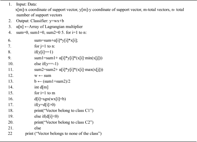
Support vector machine
The Support Vector Machine (SVM) is a popular supervised machine learning algorithm used for classification and regression. The objective of the SVM algorithm is to classify data points in an N dimensional space by finding a hyperplane14. It is considered one of the best methods for both linear and nonlinear classification. The input data of the banana leaf is classified by SVM into two distinct classes: diseased and non-diseased. Two hyperplanes, HP1 and HP2, are drawn at the borders of the two classes (Fig. 8). The Euclidean distance between the hyperplanes is then calculated. Another hyperplane is drawn so that its maximum distance from HP1 and HP2 will be the classification boundary. Therefore, the equation for the classification boundary is determined.
$$(X) \, = wTx + {\text{ bg}}$$
(7)

Let us consider a random sample x1 illustrated in Fig. 8,
If g(x1) = wt*x1+b>0 then x1 belongs to C1
If g(x1) = wt*x1+b<0 then x1 belongs to C2
In13 cubic kernels are used to classify the leaf (Kernel is basically a function which transforms the training set into a nonlinear data set). The general solution used for classification is given by
where {xi,yi} is the training set and K is the kernel function, with the value of yi as{− 1,1}4,13,46.
Convolution neural network
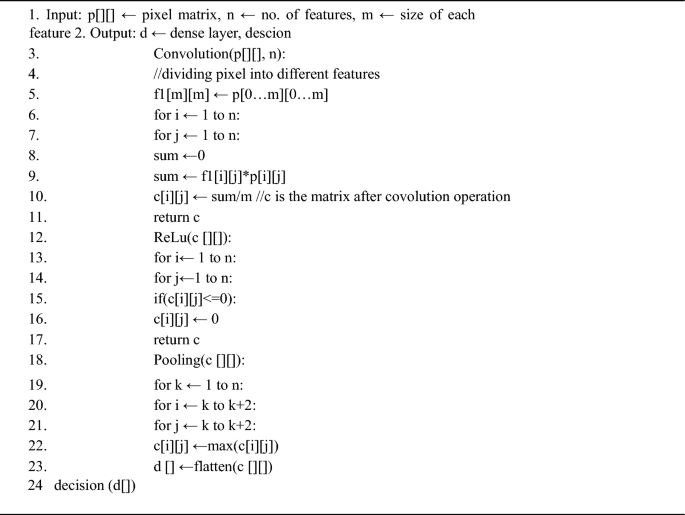
Convolutional Neural Networks (CNN) are a popular deep learning architecture used for image recognition and processing33,41. They require a large amount of labelled data for training. The input is in the form of a triplet (x,y,z), where x and y represent the width and height pixel coordinates, and z indicates the number of channels. In the hidden layer, the image undergoes convolutional, pooling, and dense layers. The image first passes through the max pooling layer, followed by a convolutional layer, and then another pooling layer. The dimensions are flattened in the dense layer. CNN utilizes the ReLu and SoftMax activation functions18,23,29. The softmax function generates the probability vector of the output layer.
$$\text{P}\left(\rm{y}=\frac{\text{j}}{\rm{x}}\right)=\frac{{e}^{{(w}_{j}^{T}+{b}_{j})}}{\sum {e}^{{(w}_{j}^{T}+{b}_{j})}}$$
(9)
The parameters in the softmax function are updated using gradient descent algorithm which is given by:
$${w}{\prime}=w-\frac{\partial J\left(w,b\right)}{\partial w}$$
(10)
$${b}{\prime}=b-\frac{\partial J\left(w,b\right)}{\partial b}$$
(11)
where \(\frac{\partial \text{J}(\text{w},\text{b})}{\partial \text{w}}\) is the slope in direction of w, and \(\frac{\partial \text{J}(\text{w},\text{b})}{\partial \text{b}}\) is the slope in the direction of b16.
The ReLu operation is piecewise linear function which is used to introduce non-linearity in the give dataset. After the convolution operation is performed, the pixel matrix has some negative values. To get rid of these values the ReLu operation is performed, by making all the values less than 0 and/or equal to 0 as shown in Fig. 9. The advantage of using ReLu activation function is achieved by not allowing the activation of all the neurons at same time. It is given by

$$f(x) = \left\{ {\begin{array}{*{20}l} x \hfill & {if\;x > 0} \hfill \\ 0 \hfill & {if\;x < 0} \hfill \\ \end{array} } \right.$$
ReLu operation is:
In the convolution layer the, firstly the features are taken from the feature extraction and the feature selection algorithms mentioned above. Then according to these features the banana leaf image is classified into different sections. The ReLu or softmax function removes the negative values1,25. The max pooling layer then tries to reduce the length of strides so that the computations become easy. For making the computations be more exact, a dense layer is added which reduces the dimensions. After all the operations are performed, next step is to classify the segments of the banana leaf into a diseased or a healthy leaf (Fig. 10). The limitation of CNN is that it cannot handle rotation3,18,51.
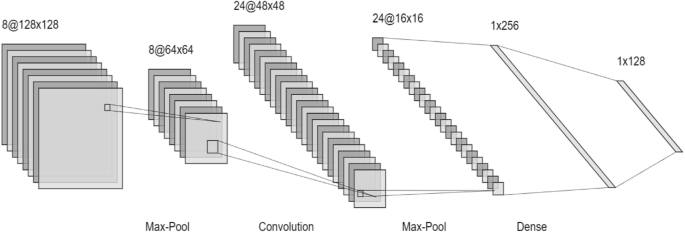
Convolution Neural Network
Artificial neural network
Artificial Neural Networks (ANN) is computational models inspired by the structure and function of biological neural networks in the human brain. They consist of interconnected nodes, or neurons, organized into layers. Information flows through the network from input nodes, through hidden layers, to output nodes, with each neuron performing a simple computation. ANNs are trained using a process called supervised learning, where they adjust the strengths of connections between neurons to minimize the difference between predicted and actual outputs. They excel at tasks such as pattern recognition, classification, regression, and decision-making, and have found widespread applications across various fields.
The input layer serves as the initial stage of the ANN, where extracted features from the images are transmitted for processing. Each feature extracted from the image corresponds to a neuron in the input layer, collectively forming the foundation for subsequent analysis.
Subsequently, the hidden layer(s) of the ANN undertake complex transformations on the input features, extracting relevant information crucial for accurate classification. These hidden layers act as intermediaries, orchestrating intricate mathematical operations to decipher the intricate patterns inherent in the input data. The design of the hidden layers, including the number of layers and neurons, is meticulously tailored to accommodate the complexity of the classification task and the nuances within the dataset.
Upon traversing through the hidden layers, the processed information converges onto the output layer, where final predictions or classifications are generated. In the case of banana leaf image classification, the output layer consists of neurons corresponding to distinct classes or categories of diseases prevalent among banana plants. For instance, neurons may represent fungal infections, bacterial infections, or nutrient deficiencies, depending on the classification schema.
Each neuron in the output layer employs an activation function, typically the softmax function for multi-class classification tasks, to produce probability distributions over the classes. This facilitates the interpretation of the network’s output, indicating the likelihood of each class for a given input image. The combined efforts of the input, hidden, and output layers synergize to empower the ANN in accurately categorizing banana leaf images, thereby contributing to the effective management of diseases affecting banana plants.


