A novel framework GRCornShot for corn disease detection using few shot learning with prototypical network

Figure 2 presents the methodology outlining the GRCornShot model’s training and evaluation process. The images of corn diseases and healthy corn are collected. After the dataset collection, the images are preprocessed, including resizing and normalizing them. These techniques are essential for the preparation of the data for training. Data augmentation techniques, such as rotation to an angle, color adjustments, and flips, make the model more generalized and flexible. These techniques bring variation to the training data. Due to this, the model can’t be overfitted. This work introduces a robust approach for corn disease detection by integrating Gabor filters with ResNet as a backbone network and utilizing a Prototypical Few-Shot Learning framework. The proposed method aims to enhance feature extraction, particularly focusing on the texture variations in diseased corn leaves, and addresses the challenge of limited labeled data for agricultural disease diagnosis. This network extracts the features from the input data, which a few-shot learning models further use. Prototype Computation is related to the prototypical few-shot learning technique, in which the prototype is calculated for each class by extracting the features from the support set images and then averaging the feature embeddings. The next step after prototype computation is the query classification. In this step, the query set data is classified into different classes by comparing it to the prototypes calculated. This classification is done based on the distance between query examples and prototypes. A detailed description of these steps is discussed in the next subsections.

Benchmark datasets in plant disease detection

In this study, the dataset is carefully created by merging and enhancing publicly available corn disease datasets from the Roboflow and Kaggle platforms^50,51. These two sources offer complementary characteristics: Kaggle datasets primarily contain images captured under controlled conditions with minimal background noise, while Roboflow datasets include images with varied lighting, field backgrounds, and environmental noise, representing more realistic agricultural scenarios. To ensure a balanced class distribution, an initial data audit of both sources is conducted to analyze the number of images per disease class. This revealed a significant class imbalance, with certain disease categories being under-represented. To address this, targeted data augmentation techniques are applied, preferentially to the minority classes, including rotation, horizontal and vertical flipping, and color jittering. This augmentation process not only increases the size of under-represented classes but also improves the intra-class variability, making the model more robust to unseen data during testing. By combining samples from both structured and field-based datasets, and by applying augmentation with class-balancing objectives, potential biases in model learning are mitigated, which leads to a reduction in the risk of overfitting towards majority classes. Furthermore, a post-augmentation distribution check is performed to ensure that each class contributed proportionally during the meta-training and meta-testing phases of the few-shot learning framework.

This class-balanced, diversity-enriched dataset creates a real-world, yet manageable testbed for evaluating the GRCornShot few-shot learning model in corn disease detection.

Data collection and preprocessing

In the proposed work, the corn leaf image dataset is collected from publicly available sources: Roboflow Universe⁵⁰ and Kaggle⁵¹. It includes images representing three common corn diseases along with healthy corn leaves, offering a diverse range of visual symptoms. The original dataset consists of 1,886 images categorized into four distinct classes, providing a solid foundation for training and evaluating the proposed model. Table 3 represents the data set summary, and Table 4 represents the detailed class-wise distribution before and after augmentation, highlighting the steps taken to address initial class imbalances. The primary reason for combining data from two diverse sources is to enhance the model’s generalization capability. Each source presented variability in lighting conditions, image resolution, background complexity, and capture angles, which collectively expose the model to a wider range of data distribution scenarios. This variation helps the model learn more generalized features, improving performance on unseen test images. All images are resized to 224\(\times\)224 pixels to match the input dimensions required for the ResNet-50 backbone. Random horizontal and vertical flips with a 50% probability are applied. Figure 3 shows sample images from all four classes, capturing both controlled and field conditions. This preprocessing pipeline ensures that the model is trained on a balanced, diverse, and realistically representative dataset, thereby improving its robustness and generalization capability for real-world deployment.

Gabor-ResNet architecture

The backbone of the proposed model is based on ResNet, which is pre-trained on the ImageNet dataset and known for its deep residual learning capabilities, which mitigate the vanishing gradient problem in deep neural networks⁵². The initial layers of ResNet-50 mainly extract general low-level features like edges and shapes. However, these features are learned during training and depend on the quality of training data. Gabor filters⁵³ provide handcrafted low-level features mathematically optimized for edge and texture detection, complementing the network’s ability to learn high-level features in deeper layers. Gabor filters mimic the functioning of the human visual cortex, which is especially well adapted to edge and texture detection. Since plant disease detection often requires identifying patterns visually distinguishable by humans, Gabor filters align well with this requirement. Instead of relying on ResNet-50 to learn all relevant features from scratch, Gabor filters pre-extract key patterns (e.g., ridges, spots, striations). This would light up part of the workload at the ResNet-50 layers, making it possible to exercise the network toward mid-level and high-level abstraction. Therefore, the Gabor convolutional layer is integrated before the standard convolutional layers of ResNet to enhance the model’s ability to capture spatial, frequency, and orientation-specific features. The Gabor filter applied in this layer is mathematically defined in Eq. 1

where:

\(\lambda\) is the wavelength of the sinusoidal component, detects features of different sizes, \(\theta\) defines the orientation angle, enabling the filter to respond to features at different directions, captures patterns at various angles, \(\psi\) stands for phase offset controlling the symmetry of detected features, \(\sigma\) is the standard deviation of the Gaussian envelope which tunes the focus on local versus global features and \(\gamma\) is the spatial aspect ratio, controlling the ellipticity of the Gabor function and distinguishes between elongated (streaks) and circular (spots) features.

In the proposed model, the Gabor layer consists of 32 channels, each parameterized with unique values of

This diversity in Gabor filters allows the network to capture various texture patterns and orientations inherent in corn disease symptoms. The Gabor layer output is then passed through standard convolutional layers within ResNet to extract deeper hierarchical features. The processed feature maps are fed into the ResNet-50 architecture following the Gabor layer. The integration of Gabor filters within the ResNet blocks ensures that low-level texture features are preserved and further refined by deeper layers.

Few-shot learning and prototypical networks

Few-shot learning is a subpart of the machine learning approach used to train models with only a few labeled examples, yet it provides impressive prediction accuracy, unlike traditional deep learning methods, which often require large amounts of labeled data. Few-shot learning leverages prior knowledge gained from related tasks to adapt to new tasks with minimal data. This technique can be helpful in various applications like medical diagnosis, wildlife species identification, and plant disease detection, especially when acquiring large datasets is not feasible. Few-shot learning is based on meta-learning, which means “learning to learn.” In meta-learning, the model is trained on a series of tasks instead of individual samples, enabling it to generalize to new tasks with only a few examples. With the introduction of the Omniglot and ImageNet datasets, the concept of few-shot learning started attracting researchers’ attention. The few-shot learning process typically involves two sets of data: a support set for training and a query set for evaluation.

The few-shot learning technique is designed in an N-way, K-shot classification scenario. In this structure, N-way refers to the number of classes the dataset has to be classified, and K-shot refers to the number of examples each class has for training. For example, a 5-way 1-shot task includes five classes with one labeled example per class, while in our work, a 4-way 5-shot task is employed, where each class has five labeled examples for training. In 2017, Snell et al. proposed an architecture called Prototypical Networks, which is widely known in the domain of few-shot learning. The core idea behind Prototypical Networks is to calculate the mean embedding of all examples belonging to a particular class, known as the prototype. The prototype serves as a reference point, and distances between the prototype and query examples are calculated, determining the class to which the query belongs. Prototypical Networks use distance-based classification, such as Euclidean distance or cosine similarity, to compare query embeddings with class prototypes. The query examples are classified based on their closest prototype in the embedding space.

The proposed work employs 4-way 2-shot, 3-shot, 4-shot, and 5-shot scenarios, representing real-world situations where annotated datasets are limited. This strategy encourages the model to learn a robust feature representation by tackling mini-tasks episodes that resemble real-world few-shot tasks. During each episode, two sets are defined: Support set S with n examples for each of the m classes, and the Query set Q is used to evaluate the model’s performance with separate examples from the same m classes.The episodic approach is inspired by meta-learning principles, where the model learns to generalize to new tasks by adapting quickly with minimal data. This task-level training enables the model to handle various few-shot learning settings.

In an m-class n-sample task, the dataset can be divided into a training set S and an evaluation set Q, expressed as Eqs. (9) and (10), respectively.

where x is the input data point, c is the associated class label, n is the number of training samples per class, and r represents the number of evaluation samples from each category.

As depicted in Fig. 3, feature embeddings for the support set are generated from the input samples. Subsequently, the similarity between a query set example and the support set embeddings is measured using a distance metric, such as Euclidean Distance or Cosine Similarity. This distance computation is essential for determining how closely the query example matches each class, leading to its final classification.

For each class m, the prototype \(\textbf{c}_m\) is derived by averaging the feature representations of all support instances \(\textbf{x}\) within that class from the support set S

denotes the embedding function mapping an input example to a feature space.

Once the class prototypes are established, the model calculates the Euclidean distance between each query example \(\textbf{x}_q\) and the prototypes \(\textbf{c}_m\):

Each query example is assigned to the class whose prototype has the minimum distance to the query embedding:

To obtain a probability distribution over classes, the distance scores are passed through a softmax layer, providing the likelihood of the query sample \(\textbf{x}_q\) belonging to each class m:

For training, a cross-entropy loss function is minimized across all few-shot classification tasks:

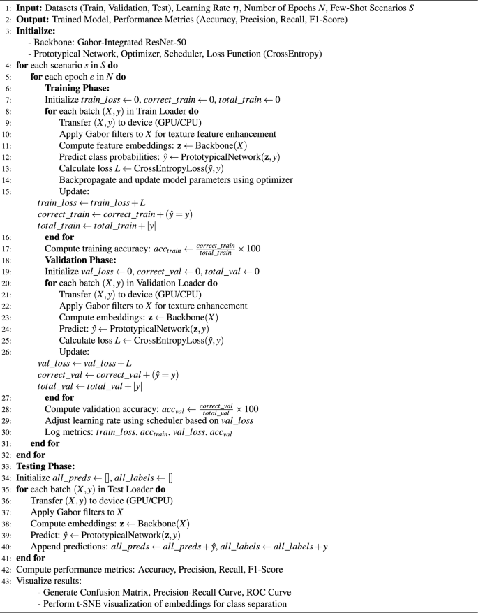
This loss function encourages the model to minimize the classification error by assigning higher probabilities to the correct class. Stochastic Gradient Descent (SGD) is used to optimize the network parameters\(,\) and the model is evaluated based on its ability to generalize across various few-shot settings. Algorithm 1 presents the training and evaluation process of the Prototypical Network using a Gabor filter-integrated ResNet-50 architecture for corn disease detection and classification.

In short, the GRCornShot model is precisely designed to overcome the difficulties of corn disease identification under sparse data availability conditions. Combining Gabor filters and ResNet-50 improves texture feature extraction for identifying disease patterns. At the same time, Prototypical Networks enable efficient few-shot classification through learning robust class prototypes from few examples. Benchmark datasets curated from Kaggle and Roboflow, with customized data augmentation and preprocessing methods, lead to better generalization of models to real-world settings. Using an episodic training and meta-learning paradigm, GRCornShot effectively addresses few-shot tasks and provides a scalable, versatile, and efficient solution for diagnosing early corn disease in agro-applications. The following section provides the experimental configuration, evaluation measures, outcome, and comparative analysis showing the efficacy of the suggested solution.