A neural signature of adaptive mentalization

Participants

The study was approved by and conducted in accordance with the policies of the Institutional Review Board of the University of Zurich and the Cantonal Ethics Commission in Zurich (study protocol 2019-00653). We recruited 506 healthy participants from the participant pool of the Department of Economics at the University of Zurich. Fifty of these completed the task while undergoing fMRI (all males, age = 23.44 ± 2.57 years), the others only performed a behavioral version of the task (56% females, age = 24.7 ± 4.7 years). To replicate our neural results and to test the generalizability of the neural signature in a more diverse sample, we also report analyses from another sample of participants that constitutes the control group of a clinical study that will be reported in a separate publication (n = 47). Notably, these participants markedly deviate from the default young student population demographic in neuroimaging research (n = 47, 57% female, age = 32 ± 8.2 years, years of education = 16 ± 3.1). For the fMRI sessions, we excluded participants ineligible for fMRI scanning according to standard MRI safety exclusion criteria. All participants gave written informed consent. To ensure sufficient power (of at least 80%, to detect moderate effect sizes with P < 0.05) and to validate and characterize the CHASE model, we chose a large sample size for the behavioral experiments, an order of magnitude larger than typical behavioral experiments. For the fMRI experiment, our chosen sample size provides sufficient power (of at least 80%) to detect moderate effect sizes with P < 0.05, which is comparable to or exceeds the average sample size of most fMRI studies^5,10.

Experimental design

Task

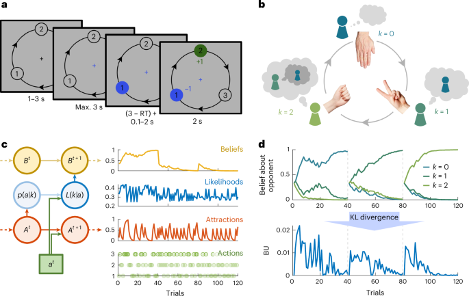
Participants played variants of repeated RPS games against human and artificial opponents. In every round, both players simultaneously picked one of three available actions (‘rock’, ‘paper’ or ‘scissors’). Each action beat one action and, in turn, got beaten by the third, leading to a circular, nontransitive dominance structure (that is, ‘rock’ beats ‘scissors’, ‘scissors’ beats ‘paper’, ‘paper’ beats ‘rock’). To reduce cognitive demands and reinforce this payoff structure, as well as to allow for a straightforward extension of the action space (that is, introducing a fourth action), we presented the game in the form of a circle where participants picked a number instead of symbols (from 1 to 3 or 4 depending on game variant; Fig. 1a). Then, the player who picked the number that was exactly one step ahead of the opponent’s number won the round (and the other player lost; choosing the same action resulted in a tie; the direction of the action dominance was indicated by arrows).

To test the robustness of our findings, we performed several experiments where we modified one or several components of the game, namely (1) the number of possible actions (3 versus 4), (2) the memory demands (by displaying the recent history in the game, the last 12 trials), (3) the used incentive scheme (zero-sum or not) and (4) the opponent (human or artificial). Across all experiments, participants were instructed that they would be randomly matched with other participants to play several matches lasting 30–40 rounds each. Participants typically played six matches (and were always instructed to meet a new opponent in each match), leading to a total of 180–240 trials (see Supplementary Table 1 with the exact specifications of the different experiments).

In the ‘discovery fMRI’ dataset, participants played against three different artificial opponent types in the scanner (with either 0, 1 or 2 steps of reasoning). Throughout each run, participants played against the same opponent type, and after each run they switched to another opponent type to avoid subsequent repetitions. Specifically, they played against each opponent twice in a counterbalanced order, leading to six runs in total. One run consisted of 40 trials, while each trial consisted of a fixation phase (0–6 s), a response phase (3–6 s) and feedback phase (2 s). Intertrial intervals (ITIs) were carefully chosen through simulations to maximize design efficiency and decorrelate action from feedback phase. On average, trials lasted around 7.3 s, with a total of 24 min of the game inside the fMRI scanner.

For the ‘replication fMRI dataset’, we collected more data by increasing the number of observations per participant (instead of scanning more participants), and thus changed the experimental timing in the replication fMRI dataset as follows. Again, participants played against three different opponent types in the scanner (with either 0, 1 or 2 steps of reasoning). However, this time, participants played thrice against each opponent, again with counterbalanced opponent type order to avoid subsequent repetitions, leading to nine runs in total. One run consisted of 40 trials, while each trial consisted of a fixation phase (1–3 s), a response phase (3–5 s) and feedback phase (2 s). Again, ITIs were carefully chosen through simulation to maximize design efficiency and to decorrelate response from the feedback phase. On average, trials lasted around 7.3 s, with a total of about 45 min of the game inside the scanner.

All games were incentivized—the final game score was converted to CHF based on predetermined conversion rates (3-to-1 for fMRI and 4-to-1 for the behavioral experiments) and paid out at the end of the experiment (in addition to a fixed show-up rate). On average, participants earned 69.4 ± 6.4 CHF in the fMRI experiment and 30.5 ± 5 CHF in the behavioral experiments.

Artificial opponents

To provide a general-purpose measure of mentalization, we aimed to (1) make sure all participants interact with behavior that is equally informative about the opponent’s strategy, and (2) test how flexibly (and quickly) participants can adapt to a range of different sophistication levels. To achieve this level of experimental control, we used artificial opponents that mimic human behavior. This approach also allowed to induce high levels of reasoning (k = 3) that earlier models of repeated strategic interactions were typically not able to capture.

To ensure that the artificial opponents are as human-like as possible, we based them on the CHASE model that we also use to explain participant behavior, as this model provided the best account of participant behavior across a wide range of game specifications in human-versus-human gameplay (see Fig. 2b for model comparison and below for a specification). In particular, the artificial opponents used the same learning rule and recursive reasoning mechanism, but were fixed to one level of sophistication (either k = 0, 1 or 2; that is, no adaptive BUs). In addition, we carefully calibrated the noise structure (when and how they deviated from their strategy) to balance informativeness and human-likeness over a series of behavioral experiments (datasets 2c and 2d; n = 134; see Supplementary Methods for details).

To confirm that the resulting artificial opponents cannot be distinguished from human opponents, we conducted a Turing-test-like assessment in three behavioral sessions. As in all behavioral experiments, participants were instructed to play against other participants who were simultaneously tested (18 participants per session) in the same room (in small cubicles for anonymity). At the end of the experiment, we asked them to rate on a five-point Likert scale whether the different opponents they played with were human or artificial. We conducted a Komogorov–Smirnov test to assess whether there are any differences between the ratings for human and artificial opponents (Fig. 2a).

The behavioral experiments took place in one of the large behavioral labs at the UZH Department of Economics, accommodating up to 35 participants per session. All experiments were fully computerized and participants were seated in individual cubicles. The computerized environment and the arrangement of cubicles ensured that participants remained anonymous, preventing them from discerning the identity of their opponents (human or artificial opponent).

In both of our fMRI experiments, participants were informed that they were competing against opponents situated in a neighboring room. They were informed that we implemented meticulous measures to ensure that participants remained unseen by one another throughout the experiment, thereby eliminating potential bias in their beliefs or behaviors. Specifically, participants were told that their opponents were located in an adjacent behavioral lab within the facility, which they passed by and witnessed when entering the scanner room (this behavioral lab room is equipped with 14 computerized cubicles for behavioral experiments). To enhance the realism of this setup, we conducted connection checks on the screen before commencing the experiment. Furthermore, at the beginning of each run, we simulated delays, suggesting that we were waiting for the readiness of other participants. This was convincingly done either through simulated telephone calls or by research assistants, indicating that we were awaiting the signal to start, thereby reinforcing the impression of a large experimental environment. Coupled with the carefully calibrated bot, which passed a modified Turing test to ensure human-like behavior, these elements collectively fostered a convincing experience of engaging in real-time competition with other human opponents.

Computational models

To link the observed behavior in the game (a series of actions) to putative underlying cognitive mechanisms and strategies, we considered and compared a series of cognitive-computational models that people might be using. These included simple learning rules (for example, reinforcement learning or fictitious play) and more complex strategies that alternate among different learning rules or propose additional mechanisms of responding to the opponent (such as experience-weighted attraction, EWA).

CHASE model

In line with earlier models of recursive reasoning^18,19,20 and related empirical findings²⁵ that humans systematically deviate from random gameplay, our proposed CHASE model assumes that players base their mentalizing on the assumption that there is a salient action that nonstrategic players (defined as k = 0) would choose more often than others. Strategic players then add a limited number (k) of recursive reasoning steps by iteratively best-responding to that action (for example, if ‘rock’ is salient, a k = 1 agent will choose ‘paper’, a k = 2 agent ‘scissors’, etc.). In addition, adaptive agents infer the level of recursive reasoning of the opponent by integrating evidence for the different levels over time. More formally, the proposed modeling approach is based on three main assumptions.

A1: nonstrategic play (k = 0) is governed by a Markovian updating rule

This updating rule maps the history of the game (past actions and rewards) to attractions \(A\left(a\right)\) for each action \(a\) at each trial \(t\), quantifying how salient or ‘attractive’ the different actions appear to be for a nonstrategic agent. In the context of the RPS under study here, we empirically identified this learning rule to be a simple delta rule over actions:

where I(a) is an indicator vector that is 1 for the chosen action and 0 for all other actions, and \(\alpha\) acts as an inverse forgetting rate that determines how quickly the agent forgets about past actions (or, equivalently, how much she is influenced by the most recent actions; Supplementary Methods). In other words, attractions here can be interpreted as a noisy representation of historical action frequencies with an exponential memory decay. These attractions are linked to the observed behavior through a softmax function \(\sigma\) with a noise parameter β, governing the extent to which agents tend to stick to the historical action frequencies or act randomly:

A2: strategic players (k > 0) use recursive reasoning

While a level-0 agent essentially ignores the interpersonal nature of the game, higher-level agents try to outsmart each other by predicting what the opponent will play, or predicting what the opponent thinks they will play, etc. Specifically, an agent with sophistication k assumes that the sophistication of the other agent is exactly one level lower (that is, k − 1) and therefore applies k steps of recursive reasoning. The resulting action probabilities are given by:

where \(\varPi\) denotes the payoff matrix of the game (specifying how combinations of actions map to payoffs for both players) and σ denotes a softmax function (as above; dropping the dependence on β for clarity). This means that strategic players start with the behavior of a nonstrategic agent and simulate how to respond to it, how to respond to that response, etc., up to their level k (notably, the level determines whose nonstrategic play acts as the starting point—odd levels are other-referential while even levels are self-referential). A softmax function is used here instead of argmax to incorporate stochasticity, capturing noisiness in action selection and recursive reasoning.

A3: adaptive players (\({\boldsymbol{\kappa }}\) > 1) try to infer the level of the opponent

While a k = 1 agent is certain that the opponent must be k = 0 (incapable of conceiving levels equal to or higher than his own), higher-level agents face uncertainty about which level (lower than their own) the opponent is most likely playing. To adapt to different strategic players, adaptive agents thus form and update beliefs about the opponent’s level of sophistication (please note that we denote their own maximum level by \(\kappa\) to distinguish it from the current level k of a strategic agent). In particular, they use equations (2) and (3) to compute action probabilities for each possible level lower than their own, which allows them to construct a likelihood function over levels \(L({k|a})\) upon observing an opponent action \(a\)^Opp:

Then, they use this likelihood to update their beliefs \(B(k)\) about the level of the opponent, based on their priors from the previous trial, using Bayes rule:

Finally, adaptive agents form an integrated prediction over the most likely opponent action, weighted by the belief distribution over the opponent’s level \(B(k)\), and noisily best respond to it:

In other words, for each possible opponent level \(k < \kappa\), they consider what the opponent would play and weight this prediction by their belief that this is the opponent’s true level. This approach enables a dynamic assessment of a player’s time-varying strategy at any given point in time. Notably, it also allows for a quantification of the extent of opponent-level BU, given by the KL divergence between successive belief distributions (‘Parametric modulators’).

Loss sensitivity and learning differences

In addition to these main assumptions, we add two more deviations from rationality in the recursive reasoning process. First, to allow for efficient exploration of strategies, we allow for an unequal weighting of wins and losses by introducing a parameter \(\lambda\) that scales the influence of losses in the payoff matrix (that is, the −1 entries; please note that the effect of this parameter is distinct from loss aversion in standard risk-taking tasks; Supplementary Results):

Second, we allow for individual differences in the ability to learn about the opponent’s level by distorting the likelihood function according to a softmax function, where the magnitude of distortion is determined by an inverse temperature parameter \(\gamma\) that captures the participant’s sensitivity to evidence about the level of the opponent:

This distorted likelihood function is hence used in the BU in equation (5) in place of the undistorted likelihood \(L({k|a})\).

Free parameters

In total, the resulting model is thus characterized by the following five parameters: \(\alpha ,\beta ,\gamma ,\lambda\) and \(\kappa\) (regulating the speed of updating attractions, recursive reasoning noise, sensitivity to evidence for opponent’s level, loss sensitivity and depth of mentalization ability, respectively). We verified that all parameters are identifiable by performing parameter-recovery simulations (r from 0.73 to 1 between generating and recovered parameters; see Supplementary Methods and Supplementary Fig. 3 for details).

Alternative models

Reinforcement learning (RL)

A simple nonstrategic learning rule is to repeat the actions that were successful in the past. Such an RL rule can be modeled by a delta rule of the form:

where \(\pi\) denotes the payoffs that the agent would have received for all possible actions, given the opponent action (but please note that only the payoff of the chosen action is taken into account in the update, due to the indicator vector)⁷. Here the attractions \(A(a)\) act as estimated action values (sometimes denoted Q values in other models). As for a level-0 agent, the behavior of an RL agent is then probabilistically governed by these attractions according to a softmax function, given some inverse behavioral decision temperature β:

Of note, this agent can be seen as a special case of our CHASE model that uses RL as learning rule and has \(\kappa =0\) (that is, equivalent to k = 0).

Fictitious play (FP)

A more sophisticated approach that acknowledges the agency of the other player is given by fictitious play (FP)²⁷. Here agents try to estimate the probabilities with which the other player chooses their actions and then best respond to them. This agent corresponds to a CHASE model as formulated above with \(\kappa =1\) (that is, equivalent to a fixed k = 1). Both FP and RL are fully specified by two free parameters (a learning rate \(\alpha\) and a behavioral temperature parameter \(\beta\)).

Experience-weighted attraction (EWA)

As there is evidence for both RL and FP in many games, the experience-weighted attraction (EWA) model was introduced to hybridize the two. In brief, this is achieved by introducing a parameter \(\delta\) that quantifies the extent to which an agent also learns from ‘foregone’ payoffs (that is, the payoffs that would have resulted from choosing different actions). In addition, there are two more parameters that govern the extent to which old information is discarded—a forgetting rate that is fixed and cognitively determined, \(\phi\), and one that is strategic, \(\rho\), to allow discarding old experience when needed, for example, in changing environments. In full, the update equation takes the following form:

where \(n\) captures the amount of experience (or the ‘experience-equivalent’) of the agent, which in turn is updated by:

As for the other models, attractions are converted into action probabilities based on a softmax function. The original formulation has five free parameters (\(\delta ,\phi ,\rho\) as well as initial attractions and experience-equivalent). However, to ensure stable parameter estimates, we only estimated parameters that govern the updating process, while we manually set the initial values for attractions and experience-equivalents (as we did with all other models—zero for experience-equivalents, uniform for action frequencies and expected rewards based on random opponent behavior for value estimates), resulting in three free parameters.

Self-tuning EWA

As the EWA model has been criticized for its high number of free parameters, a simplified version that fixes some parameter values to empirical values and replaces others with functions of experience has been proposed²⁸. In particular, a change-detector function \(\phi
(13)