Weather station data
Weather station data were compiled for the study area between latitude 37°N and 35°S and longitude 17°W and 51°E covering eleven IPCC’s climate reference regions19 of the African continent. For precipitation weather stations, we rely on a global database generated by Castellanos-Acuna and Hamann15. For temperature weather station records for Africa we carried out a similar data compilation, data cleaning and quality control effort as described in detail by Castellanos-Acuna and Hamann15. Briefly, data from seven public databases3,20,21,22,23,24,25 were merged (Table 1), and duplicates were removed using the enhanced master station history report (EMSHR) and its vector layer26,27. Recorded station elevations were then compared to a digital elevation model (DEM) to identify unit errors (feet vs. meters) as well as potential location errors. Generally, stations with large elevation errors in mountainous regions were retained, but stations with large elevation errors in areas of flat topography were removed due to probable location errors. Missing and zero elevation values were replaced by the DEM value.
Next, stations were ranked based on the length of the station records and their overlap with the 1961–1990 normal period, for which our baseline interpolations were carried out. Tier-1 stations had at least 27 years of records (90% of a normal period) for the 1961–1990 period, and tier-2 stations had at least 27 years of records for the 1951–1990 period. Tier-3 stations also had at least 27 years records for the 1951–2000 period. Finally, tier-4 stations had at least 15 years of records at any time from 1901 to 2020. The proportion of tiers in the final database was 35%, 9%, 11%, 45% for tiers 1 through 4, respectively. Missing values for the 1961–1990 period were then calculated using the anomaly (change factor) approach relative to CRU-TS time series data and adjusted accordingly as described in Castellanos-Acuna and Hamann15. If station records reported only average temperature, the average minimum and average maximum monthly temperatures were inferred from the interpolated diurnal range of CRU-TS time series data. Lastly the 1961–1990 normal estimate was obtained by averaging observed and estimated monthly climate values for this period.
Lastly, we filtered stations by location, only retaining the highest-tier station per rounded 0.1 decimal degree (approximately 10 km grid cell size) and within the same 250 m elevation interval were retained. This ensured removal of lower quality station data where better records were available in close vicinity. Following this quality control process, we retained 1588 stations with temperature records and 4510 stations with precipitation records (Fig. 1). The discrepancy in counts between temperature and precipitation records is common, and arises from agricultural and meteorological programs historically prioritizing collection of precipitation data over temperature data for managing water resources, understanding irrigation needs, assessing flood risks, etc.

Distribution of 4625 weather stations compiled for the database. Blue stations have records for only precipitation measurements and red stations have records for both precipitation and temperature measurements for the 1961–1990 period. A three degree checkerboard pattern, used to split data for independent validation is also shown.
Thin-plate spline interpolation
A first approximation of monthly climate grids was generated with thin-plate spline interpolation, performed using the fastTps() function of the fields package28 for the R programming environment (R). As a first approximation of general, location and elevation-dependent climate patterns, the interpolation was carried out on weather station data binned by three degree latitude and longitude grid cells and 250 m elevation classes (i.e. a 3D grid), with the predictor variables being the average latitude, longitude, and elevation of weather stations per 3D grid cell. This coarse 3D grid was chosen to initially only model general spatial patterns that were minimally influenced by outliers or erroneous station records. For computational efficiency, the aRange parameter, which controls the range of influence for the thin-plate splines, was set to 2,000 km. The R code for the TPS model used is provided in the Figshare repository29.
Although the thin-plate spline method would in principle allow more predictor variables to be specified in the interpolation model, this approach is computationally demanding, and it would also need to be carried out on original weather station locations to capture interactions among multiple factors, simultaneously raising model complexity and the size of the dataset to be fitted. Instead we use deep neural networks, which have practically no limitations regarding model complexity and database size, to fine tune the initial interpolated climate grids with the help of additional predictor variables reflecting topographic and geographic information, such as aspect, slope, distance to coast and lakes, in combination with monthly wind direction and strength obtained from general circulation models (Fig. 2).
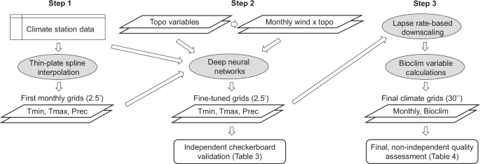
Visual summary of the novel 3-step methodological approach to climate interpolation. Thin-plate splines allow for a first approximation of monthly climate variables (Step 1). Subsequently, deep learning approach model orographic precipitation, rain shadows, lake and coastal effects (Step 2). Lastly, lapse-rate based downscaling is applied to generate high-resolution grids of monthly, seasonal, and bioclimatic variables.
Predictor variables (features)
Predictor variables, also referred to as features by the machine learning community, were generated with Spatial Analyst Tools in ArcGIS30 from a 2.5 arcminute resolution DEM (the target resolution of climate grids), which was derived from GTOPO30 data31,32. As potentially useful covariates besides latitude, longitude and elevation, we calculated a north-south directional hill shade, a topographic position index (TPI), which is a numerical index that describes ridges (high values), valleys (low values) and flat areas (intermediate values). A compound topographic index (CTI) is similar to TPI, but identifies valleys and ridges with a hydrological approach, where areas of convergence receive high values. The predictor variables Elevation, CTI and TPI were first transformed to be approximately normally distributed (log transformation with an appropriate constant), while the north-south directional hill shade was subjected to a bi-directional log transformation, separately for negative north-facing values and positive south-facing values to mitigate long-tailed variable distributions. Subsequently all variable values were re-scaled from 0 to 1.
Further, topographic variables weighted by wind direction were generated in a two-step process, that calculated directional exposure of geographic features, which were then scaled by average monthly wind direction and strength for the 1961–1990 period obtained from the Modern-Era Retrospective analysis for Research and Applications, Version 2 (MERRA-2)33.Westward and southward exposure of mountains was approximated with hill shades (45° angle with a 180° or 270° azimuth). Directional lake and coastal influences were generated with an equivalent “topography”, derived from a 2.5 arcminute grid representing lakes or oceans with a value of 1, versus land represented by a value of 0. The grid was repeatedly subjected to a 3 × 3 low pass filter to the desired range of putative lake or ocean effects (approximately 10, 50, 100 and 500 km). Directional information of distance to lake shores and coast lines were generated with hill shades as described for mountains above (180° & 270° azimuth). Both topographic and distance to waterbody “hill shades” were subsequently scaled from + 1 (e.g., maximum westward mountain exposure, or minimum westward distance to lake or coastline) to 0 (flat topography or beyond maximum distance to waterbody), to –1 (equivalent in opposite direction) and multiplied with MERRA-2 monthly wind direction and strength, provided respectively in north-south and east-west direction. To generate a single exposure layer from two directional layers, we used the geometric mean of east-west and north-south directional effects (geometric mean to avoid an overestimate of where north-south and east-west exposures overlap). The resulting grids (12 exposure layers representing each month of the year) were then again re-scaled from 0 to 1 for machine learning.
We note that deep neural networks are generally sensitive to transformation and scaling of training data, with even distributions and scaling as described above essential for good neural network performance for multiple reasons. Predictor variables need to scale with the initial random weights at a ratio of around 10:1 to achieve initial convergence and gradient decent; consistent variable scaling also prevents saturation of activation functions; and uniform initial weighting of predictors provide an unbiased starting point for training. That said, these are only consideration to improve computational performance and optimal convergence. Neural networks have no assumptions with regards to the shape of relationships of predictor and response variables or their interactions.
As an additional modification, different versions of predictor variables were generated by subjecting them to low-pass filters of 3 × 3, 5 × 5, 7 × 7, 9 × 9 and 15 × 15 grid cells of the 2.5 arcminute target resolution. The rationale for these predictor variable versions is that topography and atmospheric circulations interact at different scales. For example, rain induced by orographic lift in mountainous regions takes place at the height of cloud layers and therefore does not closely track minor topographic variation at the ground level. Because the optimal scale is unknown, we generated a range of scales for predictor variables that were evaluated through neural network importance values (based on their empirical usage in neural network weights). Although in our study, neural network predictions were not sensitive to the exact selection of variables, variable importance values nevertheless varied for different variables in different months. For data processing and programming efficiency, we used a first pass of deep neural network training on a limited set of variables to guide the selection of predictor variables that was used for development, training and prediction of all variables, listed in Table 2, and with some examples shown in Fig. 3.
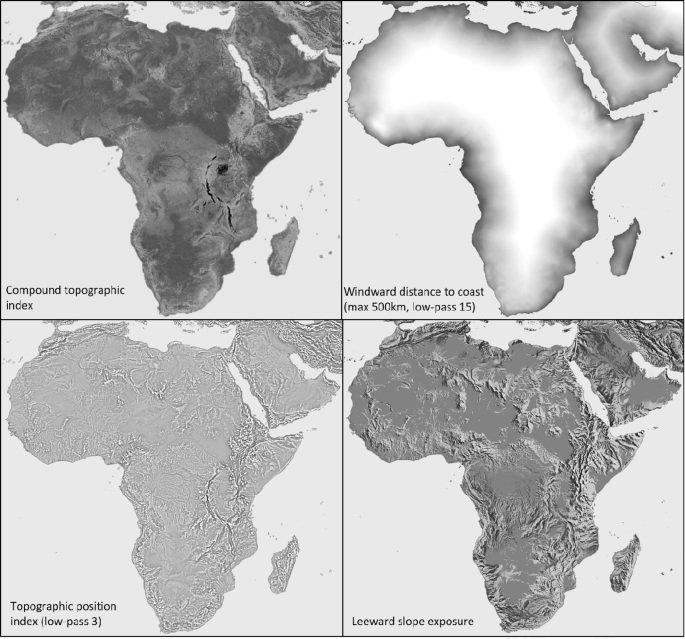
Example of predictor variables used in neural network fine-tuning of thin-plate spline interpolations. All putative predictor variables were subjected to transformations for normality if possible, and then scaled to values between 0 (black) and 1 (white) for use as covariates in deep neural network models.
Fine tuning with deep neural networks
Deep neural network methodology was applied to fine-tune the thin-plate spine interpolation with a larger dataset of predictor variables (Table 2), including all predictor variables for the location of weather stations, and the climate records of stations as dependent variable. We used the Keras package for R34 as a front end to define the neural network architecture, and the DALEX package35 to evaluate the importance of predictor variables in the neural network model. The computational work was executed on Google’s Tensorflow machine learning platform on an Nvidia’s RTX A2000 graphics card in Python. Our network architecture is an approximately 3 million parameter model that can execute training and prediction of a single variable for a continent in about 15 minutes on a modern mid-level consumer graphics card. Note, that software and package compatibility is version-sensitive. As of 2024, a compatible software chain comprises Anaconda v.2022.10 with Python v.3.9.13, Tensorflow v.2.10.1, Nvidia’s cuDNN v.8.1.0 library, the CUDAtoolkit v.11.2 for Python. This computational back-end is compatible with R v4.4.x and Keras (for R) v2.13.
The neural network architecture we used was a feed forward model that was empirically optimized by varying model parameters, and observing the resulting changes in the evolution of validation statistics throughout the training period, using an initial 80:20% random training:validation split. Model parameters that were varied included the number of hidden processing layers in the neural network (1 to 10 processing layers were tested), the number neurons per layer (8, 16, 32 … 4096 neurons per hidden layer), and increasing, decreasing or fixed numbers of neurons from first to last processing layer. As counter-measures to over-parameterization, we tested the inclusion of dropout layers where a proportion of neurons are re-set to a zero-activation state in specific intervals during training, as well as kernel regularization, which imposes constraints on the maximum value of the network weights in a processing layer.
As a general network architecture that worked well for all climate variables, we arrived at a relatively large first hidden layer, given a small set of 27 predictor variables, comprising 2048 neurons but that required an L2 kernel regularization, followed by a dropout layer (rate = 20%) and seven subsequent processing layers, each half the size of the proceeding layer (1024, 512, … 16 neurons). A number of standard hyperparameter choices that generally work well for feed forward network architecture proved satisfactory for our models as well: the ReLU activation function, which introduces a non-linearity into the model, a mini batch size of 32, which represents the number of stations processed at once before network weights are updated, a learning rate controlled by the Adam optimization function, and the mean absolute error as loss function, which is less pensive to outliers than the mean squared error. The implementation of this architecture with the Keras package for R is provided in the Figshare repository29. The wide initial processing layer allows the model to account for a variety of different local weather patterns found throughout the continent, without requiring spatial stationary in predictor-response variable relationships.
Over-parameterization was also controlled by the number of epochs (number of passes through the entire training dataset), which was set individually for each climate variable, ranging from 75 to 500. The tendency to overparameterize was first evaluated with a random 80% training and 20% validation data split (specified as a parameter in the neural network architecture in the Keras package). However, this type of validation is not entirely independent due to spatial autocorrelations among nearby weather stations. For an additional independent validation, we used the “checkerboard” method used for the development of WorldClim2 with a 3 × 3° grid to assign stations to cross-validation groups, delineated by their geographical coordinates falling within either a “black” or “white” tile (Fig. 1). This ensured that testing data were spatially distanced from training data, and the maximum epoch size for network training was set to where no further improvements were observed in validation statistics.
Climate variables and historical periods
Climate variables include 48 monthly variables: mean minimum temperature (Tmin01 to Tmin12), mean maximum temperature (Tmax), monthly average temperature (Tave) and monthly precipitation (Prec). Bioclimatic variables include mean annual temperature (MAT), seasonal 3-month totals for precipitation (e.g. PrecDJF, PrecMAM, etc.), and 3-month means for maximum temperature (TmaxDJF, etc.), minimum temperature (TminDJF, etc.) and average temperature (TaveDJF, etc.), mean warmest month temperature (MWMT), mean coldest month temperature (MCMT), temperature difference (TD = MWMT-MCMT), mean annual precipitation (MAP), growing degree-days above 5 °C (DD > 5), heating degree-days below 18 °C (DD < 18), cooling degree-days above 18 °C (DD > 18), Hargreaves’ reference evaporation (Eref), and Hargreaves’ climatic moisture deficit (CMD). The calculation or estimation of these variables is described in detail by Wang, et al.13.
Also as described in detail by Wang, et al.13, we use a change factor approach to derive high-resolution historical time series of monthly, annual, decadal, and 30-year normal climate data for the last 120 years (1901 to present). Historical anomaly layers relative to the 1961–1990 normal period were developed from the Climatic Research Unit gridded Time Series (CRU-TS) v.4.053 at a 0.5° grid size, corresponding to approximately 50 km resolution. Climate variables at this relatively coarse resolution are expected to be less accurate, especially in mountainous terrain. However, by converting the CRU-TS climate estimates to anomalies and downscaled by the ClimateAF software package, historical data can be generated with statistical precision comparable to high-resolution climate normal layers13. Storing only one high-resolution baseline climate grid, and 120 annual low-resolution anomaly layers (1901–2020) reduces the total database size by two orders of magnitude, with minimal sacrifice to statistical accuracy, even in complex terrain13.
Future climate projections
Similarly, future climate projections can be generated by the software, using the same change-factor approach, which in this case also serves as an effective bias correction method for AOGCM estimates13,16. We used thirteen CMIP6 models, based on the six criteria used by Mahony, et al.16. Briefly, we required models to have a minimum of three historical runs, low bias relative to historical runs, and availability of estimates for both mean daily minimum temperature and mean daily maximum temperature and projections based on a complete set of future emission scenarios. In model selection, we also avoided to choose more than one model from the same institution, or otherwise closely related models. The 13 models included were ACCESS-ESM15, BCC-CSM2, CanESM5, CNRM-ESM2-1, EC-Earth3, GFDL-ESM4, GISS-E2.1, INM-CM5.0, IPSL-CM6A-LR, MIROC6, MPI-ESM1.2-HR, MRI-ESM2.0, UKESM1-0-LL. We use all SSP scenarios that were consistently available for the above models, which were SSP1-2.6, SSP2-4.5, SSP3-5.8 and SSP5-8.5. For more details about these models and the selection process, see Mahony, et al.16.
The selected 13-model ensemble had an average Equilibrium Climate Sensitivity (ECS) of 3.7 °C, with a variability spanning from 1.9 °C to 5.6 °C. This aligns with the ECS values derived from the complete CMIP6 ensemble, which also stands at 3.7 °C, with a range from 1.8 °C to 5.6 °C36. To arrive at recommendations for model ensemble subsets for Africa and its 11 IPCC climatic subregions19, candidate models were further narrowed down based on four additional criteria by Mahony, et al.16, including the requirement of an equilibrium climate sensitivity between 2 and 5 °C to avoid outlier models in a smaller set, a sufficiently high model resolution, a higher number of simulation runs, and low spatial anomalies in projections (excluding BCC-CSM2-MR, IPSL-CM6A-LR INM-CM5.0 and CanESM5 for regional ensemble recommendation). However, we made an exception for UKESM1-0-LL, which was retained as one (optional) representative of a highly sensitive projection.
To obtain ordered ensemble subsets, the remaining models (8 or 9 if including UKESM1-0-LL) were subjected to the KKZ algorithm37 to maximize multivariate representation of variability in future projections for a user-selected number of models as described by Cannon38. The KKZ algorithm orders the models with the first selection closest to the ensemble centroid, the second selection being most distant from the first, and the third and all subsequent selection being most distant to previously selected models in multivariate climate space. The procedure is sensitive to selecting outlier scenarios as the second selection, which is why we restricted the sensitivity of candidate scenarios (with an optional exception to include UKESM1-0-LL).