A fully automated classification of third molar development stages using deep learning

In this section, we discuss the data set preparation in this study and introduce the neural network model used for data analysis, while proposing a comprehensive automated methodology that combines Region of Interest (ROI) extraction, carefully selected pre-filtering, and extensive data augmentation techniques. We provide quantitative measures utilized to verify the validity and performance of the study and emphasize key image attributes to improve classification accuracy significantly. Validation metrics and our strategy utilizing a variety of deep neural network architectures, including EfficientNet, EfficientNetV2, MobileNet Large and Small, ResNet18, and ShuffleNet, all optimized for this specific task.

Preparing the data set

In this research, we conducted a retrospective study utilizing archived data. All data used in the study was deidentified to ensure confidentiality. The University of Illinois Chicago’s Office for the Protection of Research Subjects (OPRS) Institutional Review Board (IRB) granted an exemption from the requirement for informed consent, providing IRB-exempt status to the study with the assigned Study ID: (2021-0480), all methods were performed by the relevant guidelines and regulations of the University of Illinois Chicago’s OPRS and IRP. We performed a comprehensive analysis of Orthopantomograms (OPG’s) and accurately classified them based on the different stages of tooth development using the Demirijian tooth development stages as a reference. Our approach involved meticulous examination of various images to ensure precise classification⁶. To conduct this study, two skilled practitioners meticulously reviewed more than 15,000 orthopantomograms (OPGs) from the patient records database of the University of Illinois, Chicago, College of Dentistry clinics, and implemented a rigorous pre-filtering process. The sample exclusion criteria comprised poor image quality and the lack of essential demographic information. Furthermore, patients with dental or craniofacial anomalies, as well as those affected by syndromes impacting dental or craniofacial structures, were excluded from the study. Additionally, individuals with a history of head and neck trauma or prior head and neck surgery were also excluded. The established protocols and careful handling of the data collection process were designed to ensure its reliability and validity. The OPGs were labeled as the follows: (1) Missing lower 3rd molar. (2) Empty Follicle and the Demirjian Stages are as follows: (3) Stage A: Cusp tips are mineralized but have not yet coalesced. (4) Stage B: Mineralized cusps are united so the mature coronal morphology is well-defined. (5) Stage C: The crown is about half formed; the pulp chamber is evident and dentinal deposition is occurring. (6) Stage D: Crown formation is complete to the dentinoenamel junction. The pulp chamber has a trapezoidal form. (7) Stage E: Formation of the inter-radicular bifurcation has begun. Root length is less than the crown length. (8) Stage F: Root length is at least as great as crown length. Roots have funnel-shaped endings. (9) Stage G: Root walls are parallel, but apices remain open. (10) Stage H: Apical ends of the roots are completely closed, and the periodontal membrane has a uniform width around the root. The principal evaluator conducted a second round of classification two weeks later to assess intra-examiner reproducibility for the Demirjian classification stages, employing weighted kappa (wk) as a measure. The intra-examiner agreement demonstrated near perfection (wk = 0.92). Additionally, a separate evaluator repeated the classification process, revealing strong inter-examiner agreement (wk = 0.90). Both the evaluators are experts, clinician-scientists.

In this research, we focus on classifying wisdom teeth in panoramic images, specifically using the third and fourth quadrants (Q3 and Q4). Since the region of interest (RoI) is localized around the wisdom teeth, utilizing the entire panoramic image is unnecessary for image classification. Therefore, we aim to extract the RoI through image cropping. Figure 1 shows a panoramic X-ray image sample from our data set. We draw two rectangles over two wisdom teeth located in the third and fourth quadrants. As depicted in Fig. 1, the wisdom teeth are accurately highlighted, cropped, and resized to a standardized dimension of 192 × 192.

The final training dataset consists of 3422 OPG, each classified and curated by the primary evaluators. This data set includes both Q3 and Q4 regions extracted from panoramic images, resulting in a collection of 6624 images available for analysis. Among these images, we observe distinct distribution patterns, with 674, 734, 1160, 1062, 870, 593, 410, and 1121 cropped images corresponding to Demirjian stages 3, 4, 5, 6, 7, 8, 9, and 10, respectively. Demirjian stages are illustrated in Fig. 2. We present cropped and resized ROI of wisdom teeth taken from each class.

One important consideration regarding the data set is the potential imbalance in sample distribution across different classes. To address this issue, two effective strategies can be employed: data augmentation and weighted data sampling. Data augmentation is a widely used technique that helps to overcome model overfitting by generating additional samples during each iteration of model training. In this study, we apply various augmentation methods such as rotation, auto contrast, and translation to diversify the data²¹. These techniques introduce subtle variations to the existing samples, effectively expanding the data set. Furthermore, to ensure a balanced representation of each class during both training and testing, we implement a weighted data sampler²². The weighted data sampler assigns higher probabilities to underrepresented classes, which ensures that the model encounters a similar number of images from each class during the training process. This approach helps prevent bias towards classes with larger sample sizes and allows the model to learn from the entire data set more effectively, ultimately leading to improved classification performance. By utilizing data augmentation and a weighted data sampler, our model becomes more robust and better equipped to handle the imbalanced data distribution inherent in medical imaging tasks.

The data partitioning for training and testing is carefully performed, ensuring a robust evaluation of the proposed approach. Specifically, 5300 images are allocated for training the model, while the remaining 1324 images are reserved for testing and validation.

Deep neural networks used in this study

The Convolutional Neural Network (CNN) is one of the most efficient and commonly used trainable models for image classification tasks. It has proven to be highly effective in categorizing images into specific classes, making it a fundamental tool in various computer vision applications^23,24,25,26. The underlying principle of CNNs lies in their ability to leverage 2-D convolution operations, which allow them to extract meaningful information from images. These convolution layers act as feature extractors, capturing important patterns, textures, and structures present in the input images.

In recent years, the field of computer vision has witnessed remarkable advancements, and numerous Convolutional Neural Network (CNN) architectures have emerged, each aiming to achieve higher accuracy on large benchmark datasets²⁷. Given the context of limited data availability and the preference for smaller models due to their efficiency in training and inference, our selection of CNN architectures was strategic. Models like EfficientNet, MobileNetV3 (Large and Small), and ResNet18 are known for their compact architecture and computational efficiency, making them ideal for scenarios where data is scarce. Furthermore, these models lend themselves well to transfer learning approaches by leveraging pre-trained weights from these models, which were originally trained on large datasets, we can fine-tune them on our specific, smaller dataset to achieve significant improvements in performance. This strategy harnesses the learned features from vast, diverse datasets and applies them to our niche task of classifying tooth development stages. Among these architectures, ResNet is a standout architecture known for effectively addressing the vanishing gradient problem in deep CNNs. By introducing residual connections, information flows directly through the network, enabling ResNet to be deeper, more expressive, and achieve improved image classification performance. Another significant advancement in the realm of CNN architectures is MobileNet²⁸. MobileNet models are lightweight and resource-efficient, perfect for deployment on less powerful devices like mobile phones and embedded systems. They utilize depthwise separable convolutions, which significantly reduce parameters and computations compared with traditional convolutions, resulting in faster inference times and optimal performance for real-time applications on resource-constrained devices. Similar to MobileNet models, ShuffleNet is a convolutional neural network specifically designed for mobile devices with limited computing power. This architecture employs two novel operations, namely pointwise group convolution and channel shuffle, to reduce computational costs while preserving accuracy.

EfficientNet is a groundbreaking CNN architecture that combines the strengths of ResNet and MobileNet while addressing their limitations²⁹. It introduces a compound scaling method that optimizes the depth, width, and resolution of the network simultaneously using a single scaling coefficient. This allows users to find a well-balanced trade-off between model size and accuracy, making EfficientNet versatile and efficient for various image classification tasks. The architecture incorporates depth- wise separable convolutions from MobileNet and residual connections from ResNet, resulting in state-of-the-art performance on benchmark datasets with improved computational efficiency. In this study, we primarily use EfficientNet-B0 as our base model but we also compared it with various other publicly available CNN architectures. The general architecture of EfficientNet-B0 is given in Table 1.

The model pipeline employed in our study is illustrated in Fig. 3. As a first step, we extract the Region of Interest (RoI) and remove any irrelevant parts from the panoramic X-ray images. By focusing only on the wisdom teeth region, we ensure that the model processes and classifies the most relevant information.

Once the RoI is extracted, the cropped images undergo data augmentation. This technique involves generating new samples by applying various transformations, such as rotation, auto contrast, and translation, to diversify the training data. Data augmentation helps to mitigate overfitting and improves the model’s ability to generalize to unseen images.Once the RoI is extracted, the segmented images undergo data augmentation. This technique involves generating new samples by applying various transformations, such as minor angular rotation, auto contrast adjustment, and small translations, to diversify the training data. Data augmentation helps to mitigate overfitting and improves the model’s ability to generalize to unseen images. The data augmentation applied involves three methods to enhance model generalization: slight random rotations (up to ± 10 degrees) to mimic orientation variability, automatic contrast adjustments (10% chance) to emphasize image features, and affine transformations that include translations (up to 10% of image dimensions) to simulate subject positioning variations. The augmented images are then fed into the model for classification. The model produces 8 outputs, representing the class probabilities of the input image belonging to each corresponding class. These probabilities indicate the confidence level with which the model assigns each image to a specific Demirjian stage, ranging from stage 3 to stage 10.

By utilizing this pipeline, our model effectively processes panoramic X-ray images, focuses on the wisdom teeth region, augments the data for better training, and provides accurate and confident predictions for the classification of the wisdom teeth into different developmental stages.

In the realm of medical applications, classification tasks often benefit from data-driven machine learning solutions. In these scenarios, datasets are meticulously constructed through rigorous statistical analysis of medical images. While simpler algorithms can sometimes yield satisfactory results, the superiority of CNN-based models becomes evident both in terms of performance and their capacity to reduce the need for manual intervention. These Convolutional Neural Network models, with their ability to automatically learn intricate features from the data, stand as a promising alternative, particularly in the medical domain, where precision and efficiency are paramount. By leveraging CNNs, we can enhance the accuracy and reliability of classifications while significantly minimizing the manual effort required.

Focal loss

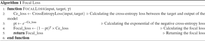
A loss function known as focal loss for handling imbalanced data was experimented with in this study³⁰. First, it calculates the entropy loss (cross-entropy loss), between the model’s predictions (input) and the true labels (target). Then it computes the probability of classification (pt) by exponentiating the negated entropy loss. Finally, it determines the loss by applying a modulating factor to the entropy loss based on the focal loss formula.

The hyperparameter γ in the focal loss formula is a tunable parameter that controls the balance between easy and hard examples during training. By the grid search approach, a value of γ = 2 yielded the best results in our experiments.

The low-pass and high-pass pre-filters

We apply a low-pass and a high-pass filter as the initial filters of our neural network structure similar to a two-channel wavelet filterbank³¹.

A Gaussian filter is a low-pass filter that smoothens an image by reducing noise and blurring unnecessary details. It is helpful for reducing noise and irrelevant features. We apply the Gaussian filter to the original 2D image and generate a new image with a focus on important features.

On the other hand, a high-pass filter complements the low-pass filter by emphasizing the high-frequency components in an image, which correspond to edges and fine details. We also apply the high-pass filter to the original 2D image and generate a new image with a focus on edges and fine details. Combining these filterbank generated images with the original 2D images adds depth to the input to the neural network. With this method, the model incorporates characteristics to obtain an understanding of the input data. This can boost the capacity of the model to identify patterns and important specifics ultimately leading to outcomes, in tasks such, as recognizing objects or classifying them. The filter parameters are listed in Table 2.

To utilize both the low and high frequency components of an image, we employ six filters, two of which pass low frequencies while the rest serve as high-pass filters. The use of multiple filters is crucial as images contain essential information that may reside in different orientations and frequency ranges. Two of the high-pass filters are known as Sobel operators, which are often employed as edge detectors for identifying edges in both vertical and horizontal directions. The original images and the resulting outputs of each filter are shown in the Appendix.

Ethics approval and consent to participate

In this research publication, we conducted a retrospective study utilizing archived data. All samples used in the study was deidentified to ensure confidentiality. “Informed consent was waived by The University of Illinois Chicago’s (UIC)Office for the Protection of Research Subjects (OPRS) Institutional Review Board (IRB)” providing IRB-exempt status to the study with the assigned Study ID: (2021-0480). All experimental protocols were approved by The University of Illinois Chicago’s IRP and OPRS