Overview of reinforcement learning agents using the Unity game engine

Reinforcement learning (learning from observation and reward) is the method most similar to how humans (and animals) learn.

Despite this similarity, it is also one of the most complex and tricky areas in modern machine learning. Quoting the famous words of Andy Karpathy.

Reinforcement learning is scary. It just so happens that everything before was much worse.

To help you understand this method, we will create a step-by-step example of an agent learning to navigate an environment using Q-learning. The text begins with first principles and ends with a fully functional example that can be run in the Unity game engine.

This article requires basic knowledge of the C# programming language. If you’re not familiar with the Unity game engine, think of each object as an agent:

• execute Start() Once at the beginning of the program,
• and Update() It runs continuously in parallel with other agents.

The repository accompanying this article is on GitHub.

What is reinforcement learning?

In reinforcement learning (RL), we have an agent that can perform actions, observe the results of these actions, and learn from the rewards/punishments for these actions.

How an agent decides to act in a particular state depends on that state. policy. policy π Functions that define agent behavior and map states to actions. Given a set of states, S and a series of actions A Policies are direct mappings. π: S → A .

Additionally, if you want to allow agents to choose from more possible options, use Stochastic policy. Then, rather than a single action, the policy determines the probability that each action will be performed in a given state. π: S × A → [0, 1].

Navigation robot example

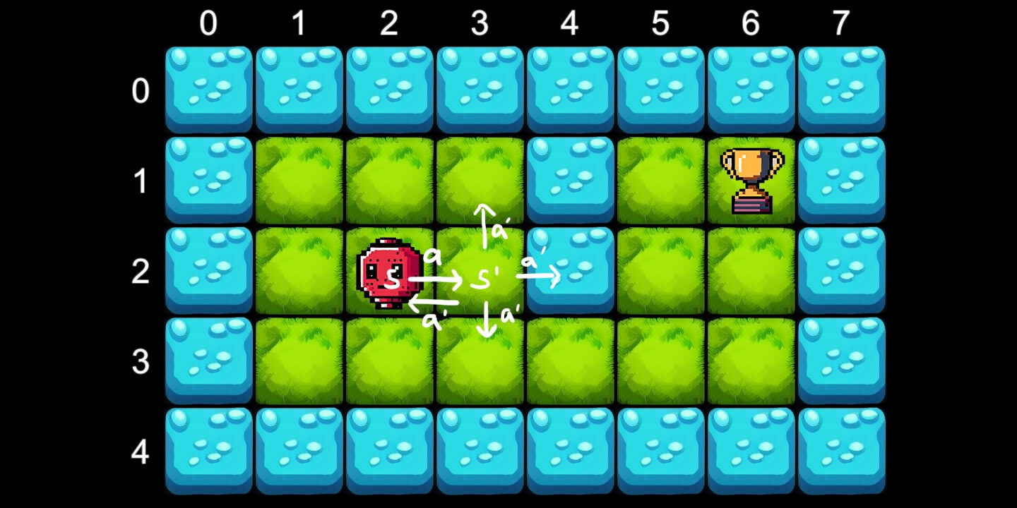
To illustrate the learning process, we will create an example navigation robot in a 2D environment using one of four actions. A = {Left, Right, Up, Down} . The robot must find its way to the prize from anywhere on the map without falling into the water.

Rewards are encoded along with the tile type using an enum.

public enum TileEnum { Water = -1, Grass = 0, Award = 1 }

State is given by position on the grid. That is, there are 40 possible states. S = [0…7] × [0…4] (8×5 tile grid), encoded using a 2D array.

_map = {
    { -1, -1, -1, -1, -1, -1, -1, -1 },   // all water border
    { -1,  0,  0,  0, -1,  0,  1, -1 },   // 1 = Award (trophy)
    { -1,  0,  0,  0, -1,  0,  0, -1 },
    { -1,  0,  0,  0,  0,  0,  0, -1 },
    { -1, -1, -1, -1, -1, -1, -1, -1 },   // all water border
}

Save map to tile TileGrid It has the following utility functions:

// Obtain a tile at a coordinate
public T GetTileByCoords(int x, int y);

// Given a tile and an action, obtain the next tile
public T GetTargetTile(T source, ActionEnum action);

// Create a tile grid from the map
public void GenerateTiles();

Utilizes a variety of tile types, so common T. Each tile has TileType given by TileEnum Therefore, the reward is also obtained as follows: (int) TileType.

bellman equation

The problem of finding an optimal policy can be solved iteratively using the Bellman equation. The Bellman equation assumes that the long-term reward of an action is equal to the immediate reward of that action. plus Expected reward from all future actions.

It can be computed iteratively for systems with discrete states and discrete state transitions. have:

• s— Current state,
• A— the set of all actions,
• s'— A state reached by taking action. a in state s ,
• γ— discount factor (the further away the reward, the lower its value),
• R(s, a)— Take action and get instant rewards a in state s

The Bellman equation states: V(s) state’s s teeth:

Solve the Bellman equation iteratively

Calculating the Bellman equation is a dynamic programming problem. each iteration ncalculate the expected future reward reachable by . n+1 Steps on every tile. Use this to save for each tile. Value variable.

Give rewards based on target tiles. In other words, 1 If the award is reached, -1 Fall into the water inside the robot 0 Otherwise. Once the prize or water is reached, no action can be taken and the state value remains at its initial value. 0 .

Create a manager that generates the grid and calculates the iterations.

private void Start()
{
    tileGrid.GenerateTiles();
}

private void Update()
{       
    CalculateValues();
    Step();
}

To track the value, VTile class that holds Value. To avoid getting the updated value directly, first NextValue Then set all the values ​​at once. Step() function.

private float gamma = 0.9; // Discounting factor

// The Bellman equation 
private double GetNewValue(VTile tile)
{
    return Agent.Actions
        .Select(a => tileGrid.GetTargetTile(tile, a))
        .Select(t => t.Reward + gamma * t.Value) // Reward in [1, 0, -1]
        .Max();
}

// Get next values for all tiles
private void CalculateValues()
{
    for (var y = 0; y < TileGrid.BOARD_HEIGHT; y++)
    {
        for (var x = 0; x < TileGrid.BOARD_WIDTH; x++)
        {
            var tile = tileGrid.GetTileByCoords(x, y);
            if (tile.TileType == TileEnum.Grass)
            {
                tile.NextValue = GetNewValue(tile);
            }
        }
    }
}

// Copy next values to current values (iteration step)
private void Step()
{
    for (var y = 0; y < TileGrid.BOARD_HEIGHT; y++)
    {
        for (var x = 0; x < TileGrid.BOARD_WIDTH; x++)
        {
            tileGrid.GetTileByCoords(x, y).Step();
        }
    }
}

value for each step V(s) The value of each tile is updated to the maximum value of all actions for instant rewards and the resulting tile’s discount amount. Future rewards are propagated outward from the reward tile, and returns are controlled in a decreasing manner. γ = 0.9 .

Quality of action (Q value)

We discovered a way to associate state and value. This is sufficient for this pathfinding problem. However, this focuses on the environment and ignores agents. As agents, we typically want to know what actions are appropriate in the environment.

In Q-learning, the value of an action is called its value. quality (Q value). each (state, action) Pairs are assigned a single Q value.

Where can I find the new hyperparameters α Defines the learning rate, or how quickly new information overwrites old information. This is similar to standard machine learning and the values ​​are usually similar. Here we use the following values: 0.005 . Then use the time difference to calculate the profit from performing the action. D(s,a):

Rather than considering all actions in the current state, we consider the quality of each action individually, so instead of maximizing all possible actions in the current state, we are calculating all possible actions in the state we will reach after performing the action, and we are combining that quality with the reward for performing that action.

The time lag term combines the immediate reward with the best possible future reward and is a direct derivation of the Bellman equation (see Wiki for details).

To train the agent, instantiate the grid again, but this time also create an instance of the agent and place it at: (2,2).

private Agent _agent;

private void ResetAgentPos()
{
    _agent.State = tileGrid.GetTileByCoords(2, 2);
}

private void Start()
{
    tileGrid.GenerateTiles();
    _agent = Instantiate(agentPrefab, transform);
    ResetAgentPos();
}

private void Update()
{
    Step();
}

Ann Agent Object has a current state QState. each QStateHolds the Q value for each available action. At each step, the agent updates the quality of each action available in the state.

private void Step() 
{
  if (_agent.State.TileType != TileEnum.Grass)
  {
      ResetAgentPos();
  }
  else
  {
      QTile s = _agent.State;
  
      // Update Q-values for ALL actions from current state
      foreach (var a in Agent.Actions)
      {
          double q = s.GetQValue(a);
          QTile sPrime = tileGrid.GetTargetTile(s, a);
          double r = sPrime.Reward;
          double qMax = Agent.Actions.Select(sPrime.GetQValue).Max();
          double td = r + gamma * qMax - q;
          s.SetQValue(a, q + alpha * td);
      }
  
      // Take the best available action a
      ActionEnum chosen = PickAction(s); 
      _agent.State = tileGrid.GetTargetTile(s, chosen);
  }
}

Ann Agent has a set of possible actions in each state, and the optimal action is performed in each state.

If there are multiple optimal actions, one of them will be executed randomly because we have shuffled the actions in advance. Due to this randomness, each training progresses differently, but typically stabilizes between 500 and 1000 steps.

This is the basis of Q-learning. Unlike, status value, quality of action Applicable to the following situations:

• Observation is incomplete at once (agent’s field of view)
• Observation changes (object moves in the environment)

Exploration vs. Exploitation (ε-Greedy)

So far, the agent has taken the best possible action each time, but this can quickly cause the agent to fall into a local optimum. A key challenge in Q-learning is the trade-off between exploration and exploitation.

• Exploit — Select the action with the highest known Q value (greedy).
• Explore — Choose random actions to discover better possible paths.

ε-Greedy Policy

give a random value r ∈ [0, 1] and parameters epsilon There are two options.

• if r > epsilon Then choose the best action (exploit),
• Otherwise, choose a random action (explore).

collapsing epsilon

Usually we want to explore more early on and get more out of it later. This is achieved through corruption epsilon over time:

epsilon = max(epsilonMin, epsilon − epsilonDecay)

After enough steps, the agent’s policies will almost always converge to select the highest quality action.

private epsilonMin = 0.05;
private epsilonDecay = 0.005;

private ActionEnum PickAction(QTile state) {
  ActionEnum action = Random.Range(0f, 1f) > epsilon
      ? Agent.Actions.Shuffle().OrderBy(state.GetQValue).Last()  // exploit
      : Agent.RndAction();                                       // explore

  epsilon = Mathf.Max(epsilonMin, epsilon - epsilonDecay);
  return action;
}

Wider RL ecosystem

Q-learning is an algorithm within the larger family of reinforcement learning (RL) techniques. Algorithms can be classified along several axes.

• State space: Discrete (e.g. board games) | Continuous (e.g. FPS games)
• Action space: Discrete (e.g. strategy games) | Continuous (e.g. driving)
• Policy type: Off-Policy (Q-Learning: a’ is always maximized) |on policy (SARSA: a’ selected by the agent’s current policy)
• operator: Value | Quality | Advantage A(s, a) = Q(s, a) − V(s)

For a comprehensive list of RL algorithms, see Reinforcement learning Wikipedia page. Additional methods such as behavioral cloning are not listed here, but are also used in practice. Practical solutions typically use extended variants or combinations of the above.

Q-Learning is a policy-independent, discrete action technique. Extending this to continuous state/action space gives rise to techniques like deep Q networks (DQNs), which replace Q tables with neural networks.

In the Grid World example, the Q table has |S| × |A| = 40 × 4 = 160 Entries — fully manageable. But for games like chess, the state space exceeds 10⁴⁴ position, making it impossible to save or fill an explicit table. In these cases, neural networks can be used to compress the information.