I thought building machine learning models required advanced mathematics, but I was wrong.

At least before the “vibe coding era,” many people lamented that they couldn’t program because they were “not good at math.” Neither did I. Anyway, here’s how I started building machine learning models in Python.

why did you hesitate

I thought that I was not good at mathematics.

Although I was interested in technology and computers, I was not good at math, at least during my formal education. I managed to pass a transferable introductory statistics course at a community college, but I felt like advanced math wasn’t for me. I became interested in Linux and tried my hand at code, but I felt like I wasn’t good enough mathematically.

Software programs like Mathematica were not in my price range. There are more open source alternatives available now, but they didn’t seem to exist when I was a student or university student, or at least I wasn’t aware of them.

The simplest code that people learn to write requires only basic arithmetic. I played around with the code and dabbled. Still, my encounter with statistics led me to see mathematics as having value in practical applications.

When machine learning became popular, I decided to give it a try. I signed up for a free course on Coursera, but without the necessary background, I quickly failed.

But one day I had the urge to try statistical programming. I used to look up math articles on Wikipedia from time to time, but there seemed to be a barrier to participation. However, when I actually tried it, I realized that it was easy to do. It also gave me a reason to teach myself math, build my own super calculator in Python, teach myself calculus and linear algebra, and even Schaum’s outlines.

Setting up the Python environment

Assemble the modeling toolbox

We needed some tools that were different from the standard Python environment. Much of statistics, data science, and machine learning in Python is done interactively. Rather than jumping straight into building a model, it’s best to explore the data and see what you can learn from it.

I have installed IPython and Jupyter. IPython is an enhanced interactive Python interpreter that adds features such as command-line editing and “magic” commands. Jupyter implements an interactive notebook for viewing and sharing your results with others. Jupyter notebooks were previously part of IPython, but the developers decided to focus on the latter, even though IPython is still used as a “kernel” in the background. Use Pixi to install and update these tools.

pandas is a library that manages data in DataFrame. This is similar to using spreadsheets or relational databases. Seaborn is a library with common statistical visualization features such as bar graphs, scatter plots, and regression plots. statsmodels provides classic statistical models such as regression. SciPy provides many scientific computing tasks, including common statistical operations.

Exploring the data

You need to know your data to model it

After setting up the environment, I needed to explore the data and build the model. First, we needed to import the Python library.

import numpy as np
import pandas as pd
import seaborn as sns
sns.set_theme()
from scipy import stats
import statsmodels.api as sm
import statsmodels.formula.api as smf
%matplotlib inline

Next, we needed data. Fortunately, Seaborn has several built-in toy datasets. One of these is a dataset from waiters that tracked restaurant bills, tips, party size, and whether there were smokers at parties over several weekends. Is there a correlation between bills and tips?

First, load the dataset using Seaborn.

tips = sns.load_dataset('tips')

This will load the dataset as a pandas DataFrame.

Let’s examine the first few lines.

tips.head()

We then obtain standard descriptive statistics such as mean, median, mode, bottom quartile (25th percentile), and top quartile (50th percentile).

tips.describe()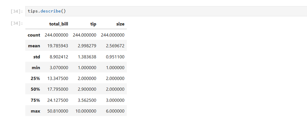

Create a scatter plot with the total amount as the independent variable on the x-axis and the tip as the dependent variable on the y-axis.

sns.relplot(x='total_bill',y='tip',data=tips)

Hmm, this scatterplot seems to have a positive linear relationship. Draw a line over these points and the tip will increase with the total amount. Although some tips are high as outliers, this relationship seems to hold in general.

You can generate a regression plot with lines like this.

sns.regplot(x='total_bill',y='tip',data=tips)

From exploration to modeling

Python makes it easy to build regression models

Now that you’ve examined your data and found a positive relationship between bills and tips, it’s time to formally model it. This is easy to do using statsmodel.

results = smf.ols('tip ~ total_bill',data=tips).fit()
results.summary()

Simply put, this creates an expression similar to that in R, and displays an overview with the model and some diagnostic information. The most useful column is the left column of the table. This includes the y-intercept and slope that you may have learned in elementary algebra class. This represents a line plotted on a scatterplot. If I were a restaurant manager, I would advise my wait staff to upsell their customers. This is because they can earn more tips and at the same time contribute to the restaurant’s profits.

This is simple linear regression taught in Statistics 101, but it’s actually a type of machine learning. This is a supervised algorithm because it fits the data to a known target, the y-values ​​of the original dataset.

This model allows you to substitute values ​​and make predictions. But what about new data? That’s where scikit-learn comes into play. This is the best machine learning library for Python. You can split your data into test and training data and make predictions. Modify and demonstrate a tutorial on regression in scikit-learn.

from sklearn.linear_model import LinearRegression
from sklearn.model_selection import train_test_split,LinearRegression
X = tips[['total_bill']]
y = tips['tip']
X_train, X_test, y_train, y_test = train_test_split(X, y)
model = LinearRegression().fit(X_train, y_train)

You can then predict hints from the “test” dataset.

y_pred = model.predict(X_test)

Modify the sckit-learn example again to plot the regression line for the training and test data.

import matplotlib.pyplot as plt

fig, ax = plt.subplots(ncols=2, figsize=(10, 5), sharex=True, sharey=True)

ax[0].scatter(X_train, y_train, label="Train data points")
ax[0].plot(
    X_train,
    model.predict(X_train),
    linewidth=3,
    color="tab:orange",
    label="Model predictions",
)
ax[0].set(xlabel="Feature", ylabel="Target", title="Train set")
ax[0].legend()

ax[1].scatter(X_test, y_test, label="Test data points")
ax[1].plot(X_test, y_pred, linewidth=3, color="tab:orange", label="Model predictions")
ax[1].set(xlabel="Feature", ylabel="Target", title="Test set")
ax[1].legend()

fig.suptitle("Linear Regression")

plt.show()

You can find this code and all others on my GitHub account.

Python does the calculations for you

Python did the math heavy lifting for us. This allows me to focus on things like wondering how effective the model is. It also motivated me to study on my own. I don’t solve matrix equations or calculate derivatives and integrals directly, but modern statistics and machine learning rely heavily on calculus and linear algebra. I have also used Python to research these topics, but that’s my own judgment. Armed with Python and your new knowledge, you will be able to explore machine learning further in the future.