From Deviation Risk to Trajectory Complexity: Machine Learning-Based Deviation Characterization and Torsion Analysis for Well Quality Assessment

Appendix 1

This appendix briefly describes the metrics used to evaluate the model.

confusion matrix

Confusion matrices are powerful tools for evaluating machine learning classification models, summarizing correct and incorrect predictions for each class. It consists of true positives (TPs) for which the model accurately predicts the positive class. True negative (TN). The model accurately predicts the negative class. False Positive (FP), or Type I error. The model incorrectly predicts the positive class. False Negative (FN), or Type II error where the model incorrectly predicts the negative class. This matrix allows visualization of the algorithm’s performance and facilitates the calculation of key metrics such as precision, precision, recall, and F1 score, which helps refine and improve the model.⁵⁰.

accuracy

The precision given by Eq. 2 is a metric that quantifies the overall effectiveness of the classification model. It is defined as the ratio of the number of correct predictions to the total number of predictions made. In other words, true positives and true negatives are combined to provide a direct measure of model performance.⁵¹.

Mathematically, precision can be expressed as:

accuracy

Accuracy is a metric that quantifies the number of correct positive predictions made. This is especially important in scenarios where the cost of false positives is high. High accuracy means that when the model predicts a deviation, it is very likely to be correct, which is desirable. Accuracy is the ratio of true positives to the sum of true positives and false positives.⁵².

Mathematically, precision can be expressed as:

recollection

Recall, also known as sensitivity, measures the proportion of actual positives that are correctly identified as positive. This is very important in situations where it is much worse to miss a positive than to falsely detect a positive.⁵².

Mathematically, recall can be expressed as:

F1 score

The F1 score is the harmonic mean of precision and recall and provides a balance between these two metrics. This is especially useful when both false positives and false negatives need to be considered. F1 score is a better measure than accuracy for models with unbalanced class distributions because it does not depend only on majority classes.⁵¹.

Mathematically, F1 can be expressed as:

ROC-AUC

An ROC curve is a graphical representation of the diagnostic ability of a binary classification system as the discrimination threshold is varied. This curve is created by plotting TP rate (TPR, also known as recall or sensitivity) against TP rate (FPR, 1 – specificity) at various threshold settings. A model that produces a curve surrounding the upper left corner of the ROC space is considered a good model.⁵³. This indicates a high true positive rate and low false positive rate across various thresholds. This means that the model can correctly distinguish between positive and negative classes with little error. In contrast, a model that produces a curve close to the diagonal of the ROC space (representing a random guess) indicates that the model is less effective. AUC provides a single scalar value that summarizes the model’s performance across all thresholds. The AUC ranges from 0 to 1, with an AUC of 0.5 indicating no discrimination (equivalent to a random guess) and an AUC of 1 indicating perfect discrimination. In general, a higher AUC value indicates better model performance, and the model is more likely to rank randomly selected positive instances higher than randomly selected negative instances.

PR-AUC

PR-AUC is a performance metric for binary classifiers that is more informative than ROC-AUC in the presence of highly imbalanced datasets. In these situations, the positive (minority) class is of great interest, and the classifier’s ability to accurately detect this class is important. A precision-recall curve plots precision on the y-axis and recall on the x-axis. Precision represents the model’s accuracy in classifying positive instances, and recall represents the model’s ability to find all positive instances in the dataset. For a model to achieve high accuracy, it must limit the number of false positives, but to achieve high recall, it must limit the number of false negatives. There is often a trade-off between these two metrics, where increasing one may decrease the other. The area under PR-AUC gives a single value that summarizes the precision and recall of the classifier over different thresholds.⁵⁴similar to ROC-AUC. However, PR-AUC is more sensitive to minority performance. This can provide a better indication of the model’s performance when positive classes are rare or when false positives are more important than false negatives.

M.C.C.

MCC is a more informative metric than other classification metrics for evaluating binary classification, especially for unbalanced datasets. This takes into account true and false positives and negatives, providing a balanced measure that can be used even when class sizes are very different. MCC is generally considered a reliable statistical rate that produces a high score only if the prediction performs well in all four confusion matrix categories.⁵⁵.

Mathematically, MCC can be expressed as:

log loss

Log loss measures the performance of a classification model whose predictions are probability values ​​between 0 and 1. The log loss increases as the predicted probability deviates from the actual label, penalizing both types of errors, but especially confident and incorrect predictions. This metric indicates the confidence level of the prediction. Useful for models that want to ensure that the probabilities of their predictions are adjusted correctly.⁵⁶.

Mathematically, log loss can be expressed as:

Appendix 2

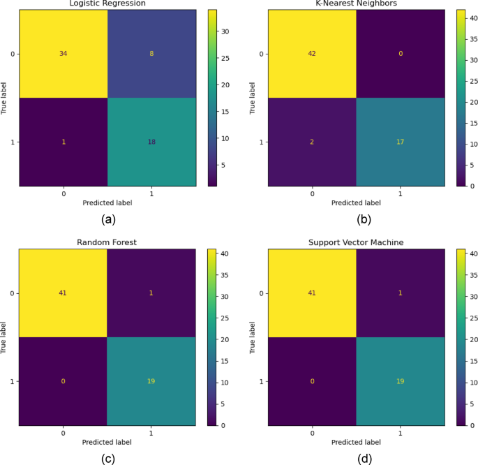
This appendix provides a concise representation of the output from four machine learning models used to predict unintended well deviations (Figures 20, 21, and 22).

To select the optimal number of neighbors in the KNN model, a 5-fold cross-validation was performed using the number of neighbors ranging from 2 to 20. The highest accuracy was achieved with two nearest neighbors. Figure 23 shows the accuracy of cross-validation for different numbers of nearest neighbors.