Vision-based tactile sensing enhanced by microstructures and lightweight convolutional neural network

Structural design and working principle

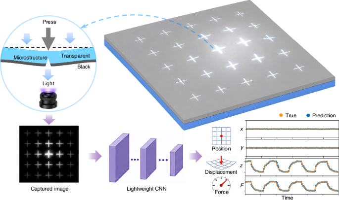
As shown in Fig. 1a, the stretchable sensor body was composed of a transparent polydimethylsiloxane (PDMS) layer and a thin black graphite/PDMS composite layer. A grid of 5 × 5 cross-shaped trench structures was precisely fabricated using ultraviolet laser cutting, with a depth of around halfway through the sensor body film (Figs. 1a and 2c). The distance between adjacent cross centres is 2 mm, with each cross measuring 1.5 mm in both length and width. The sensor body is clamped using a 3D-printed frame with a 1.6 × 1.6 cm square window. The data processing pipeline of the Micro-VBTS system, as depicted in Fig. 1c, involves image acquisition and preprocessing, followed by lightweight CNN processing to learn the patterns and features necessary for the prediction of displacement in depth (z-coordinate), applied force and location coordinates (x, y). As shown in the figure, the comparison between true values and CNN predictions demonstrates the system’s high accuracy.

Figure 2 illustrates the working principle of this Micro-VBTS sensor that leverages the deformation of microstructures to measure applied force. Initially, the laser-written trenches are nearly closed, allowing minimal light through the structure. When force is applied on the transparent side, the trench in the black layer opens, creating a clear visual feature even for very slight deformation of the overall diaphragm shape. Importantly, the optical effect is amplified by the high depth-to-width ratio of the trench. The detailed structure of a micro trench is illustrated in Fig. 2c. Images are captured by a camera under the sensor body. For instance, the images of our sensor body clearly showed distinguishable features under an applied force of only 30 mN (Fig. 1b), which indicates its high sensitivity. With the diaphragm structure and elastic sensor body, the sensor recovers spontaneously after removal of the applied force.

In this work, we focused on a cross-shaped microstructure design, which was designed to achieve efficient light modulation and enhanced deformation amplification under applied forces. Other microstructure geometries may also influence the sensing performance by altering the way light is scattered and how local stress distributions are generated. For instance, circular or square trenches, as well as hemispherical, conical, or pyramid arrays, could provide different deformation responses and image features, potentially improving spatial resolution and force sensitivity. Moreover, the choice of material, with variations in elasticity, transparency, and refractive index, could further affect both the mechanical response and optical contrast, thereby impacting the robustness and accuracy of force inference. These factors represent promising avenues for future exploration to optimise sensor performance for specific applications.

Theoretical modelling and simulation

We developed a comprehensive mathematical model to analyse the bending behaviour of a thin PDMS film with fixed boundaries and uniformly distributed V-shaped notches (Fig. 3 and Supplementary Note 1). With this model, we derived the extension of trench width (Δd) under an applied force, which is critical for modulating light transmission and amplifying the variation. This model simplifies the complex behaviour of the sensor body film by representing it as an array of fixed-fixed beams. Each beam bends independently in response to an applied load, assuming that cross-sections remain undeformed during bending. A detailed modelling process is presented in the Supplementary Note 1.

As a result, for location \(i(i\in \left\{A,B,C,D,E\right\})\), the deformations of the notch \(\Delta {d}_{i}\) (Fig. 3b) can be expressed as:

Here, \({M}_{i}\) is the bending moment at location i; \({d}_{0}\) denotes the original trench width without applied force; E denotes the effective Young’s Modulus of the film, determined through experimental calibration; \(\alpha\) is the geometric depth of the trench, also approximately half of the entire film thickness (\(h\approx 2\alpha\)) in our sensor.

To validate the mathematical model, we compared the finite element analysis (FEA) results with the analytical predictions (Fig. 3). Using COMSOL Multiphysics, we performed simulations over a range of applied loads from 0 to 80 mN, observing deformation patterns that closely matched our theoretical predictions. The applied force range was selected to represent fine-force sensing scenarios and to match the following experimental testing conditions. Further FEA was conducted (Fig. S2) to model the deformation and stress distribution of the sensor body under a 60 mN force applied at the central location. The material properties in our simulation were modelled assuming linear elasticity. The analysis revealed significant deformation around the contact point, affecting the micro trench’s luminous flux. To investigate the change of microtrench width across the 5 × 5 array, simulations were conducted for two scenarios (Fig. 3g–j): a 60 mN force applied at the central location (3,3) and at an off-centre location (2,2). Similar to our previous study³⁷, we use the average diagonal length of the quadrilateral at the cross centre to represent the deformation of the microtrench under an applied force. Figure 3g, i presents the average diagonal length at the 25 cross centres for two scenarios. Both results indicated significantly larger variation at the contact point compared to other cross centres, which results in amplified light transmission and enhanced visual features, benefiting further feature extraction.

Furthermore, the deformation results reveal that deformation patterns were radially symmetrical across the 5 × 5 array when the central location (3,3) is pressed (Fig. 3h). Locations closer to the point of contact experience greater deformation compared to other cross centres, but with less contrast compared to the average diagonal length results, shown in Fig. 3g. In Fig. 3j, where the off-centre location (2,2) is pressed, points such as (5,1), (4,4), and (5,5), which are farther from the contact point, experience less deformation compared to their counterparts when the central location (3,3) is pressed.

The simulation primarily focused on normal force application. To further demonstrate the sensor’s behaviour under more realistic contact conditions, we also included an off-axis loading scenario in which a 45° force was applied (Fig. S9). This introduces both normal and tangential force components to evaluate the microstructure’s response to shear stress and deformation. Furthermore, we conducted parametric COMSOL simulations (Figs. S6 and S7) to briefly analyse how geometric factors such as trench arm length and spacing influence local stress distributions and deformation.

Although in-plane motion and shear force tracking are not yet included, the current sensor design is theoretically extendable to multi-axis force detection through additional calibration. In fact, high-resolution tracking of lateral motion using the cross-shaped features as references is straightforward, and observing differential motion of these features would provide detailed shear information. We have not focused on this in the paper because these functions are well provided by 2D markers and may benefit less from the 3D micro-structuring. Fig. S9 shows asymmetric widening of cross arms and differential lateral motion across neighbouring trenches.These optical cues can be exploited by a vision pipeline for shear direction/magnitude estimation. These results support the potential for calibrated shear sensing in future work.

It should be noted that the 5 × 5 grid used in our experiments serves only as a calibration matrix and does not define the intrinsic spatial resolution of the sensor. Since the image patterns exhibit distinct variations even when the contact point lies between calibration crosses (Fig. S10), localisation accuracy can be further improved by adopting a denser calibration grid without modifying the physical structure. Moreover, increasing the density of microstructures or employing a higher-resolution camera could push the resolution limits further.

Experimental set-up and data collection

The fabrication of the sensor body involves two key steps: the fabrication of the multi-layer elastomer film, followed by a high-precision patterning process using ultraviolet (UV) laser cutting. During the multi-layer film fabrication, spin coating was used to ensure uniformity and precise control over the film thickness. For the laser cutting process, a high-precision UV laser cutter was employed, achieving a high aspect ratio microtrench structure with an opening width of approximately 40 μm. Detailed fabrication procedures of the sensor body are provided in Fig. S4 and ‘Methods’³⁷. According to scanning electron microscopy measurement (Fig. 1e), the total thickness of the sensor body is 1 mm, while the composite layer is ~230 μm. The depth of the micro trench was ~523 μm.

The performance of the Micro-VBTS was tested with a bespoke experimental setup, as shown in Fig. S5 and ‘Methods’. A commercial Logitech C922 camera (1920 × 1080 pixels resolution) was used to capture images at 30 frames per second (FPS) during force applications. We tested the sensor with a single contact point located at the centre of all crosses. Displacements of 0–0.5 mm, 0–1.0 mm, and 0–1.5 mm were applied against the sensor surface using a linear motor driving a cone-shaped probe (1 mm tip diameter) repeatedly at 1 Hz, with all 25 sensing points tested under consistent characterisation conditions and ambient lighting. The displacement of the linear motor was synchronously recorded. It is obvious that images captured under these conditions showed clear distinctions. The results from three typical testing points of (3,3), (1,4) and (4,4) are shown in Fig. 4b–d. The images indicate that crosses close to the contact point had high luminous flux and wide trenches, which is consistent with the modelling result. Additionally, the deformation of the film led to the displacement of crosses in images. This result was predicted by finite element simulation as well.

A quantitative image brightness-displacement analysis is shown in Figs. S3 and 4e. To investigate the sensing mechanism, we analysed the variation of optical brightness under controlled vertical displacement (z). A total of 300 video frames (30 FPS, 0–1.5 mm displacement range) were recorded while applying a vertical force at (3,3), the centre of the sensor surface. Each video frame was first cropped to a central area and then divided into 25 equally sized regions (60 × 60 pixels), forming a 5 × 5 grid. For each pixel, we extracted the value (V) channel from the HSV colour space, applied a threshold (V < 32) to suppress background noise, normalised the values to [0,1], and summed the V value of all pixels to quantify regional brightness.

Figure S3 shows the displacement–brightness scatter plots for all 25 regions. A clear monotonic trend is observed, particularly in the centre region where the force is applied. The central region (3,3) shows the steepest slope, indicating the strongest brightness modulation in response to vertical displacement. Peripheral regions exhibit smaller slope values due to less mechanical deformation.

To further quantify sensitivity, we performed linear regression on the displacement–brightness data of the central region (3,3). As shown in Fig. 4e, the slope of the fitted line reflects the local optical sensitivity to deformation. The linear fit yields the equation that \(\mathrm{Brightness}=k\times z+b=0.2676z+113.45\), where k = 0.2676 (µm⁻¹) denotes the optical sensitivity (i.e. change in brightness per unit displacement), and b = 113.45 corresponds to the baseline brightness when no force is applied. This quantification provides a clear metric for evaluating the microstructure-based brightness response to mechanical input.

This is especially beneficial for further in-depth image processing based on machine learning models to achieve high precision. Notably, while brightness is the primary measurable parameter used for sensitivity characterisation, the final machine learning model (such as CNN) can implicitly extract multiple image features beyond brightness. This enables the network to utilise global and local patterns across all 25 regions for robust prediction, rather than relying on a single high-sensitivity area.

The applied force (F) can be calculated based on vertical displacement (z-direction) based on a simple linear relationship. According to theoretical analysis and simulation³⁷, the F–z relationship can be approximately expressed as \(F\left(z\right)={k}_{{xy}}\times z\), where the coefficient k_xy represents the proportionality between vertical displacement and the applied force at location (x,y). To calibrate the coefficient k_xy, we measured the applied force with a high-precision scale (MAXREFDES82, Analog Devices Inc.), as described in ‘Methods’. As an example, the displacement results from the point (3,3) are shown in Fig. 4f, g. According to the measured force and probe displacement, a linear curve fitting was performed, and the resulting k₃₃ value was calibrated as 85.4 mN/mm. The coefficient of determination R² was calculated as 0.99 at this point, which validated that the linear model is a good approximation of the force–displacement relationship, as shown in Fig. 4h.

CNN model architecture and evaluation

We have developed an ultra-light CNN model architecture to infer the location and magnitude of applied force, as shown in Fig. 5. The CNN model was selected because of its strong capability to extract spatial features from images, making it highly suitable for vision-based tactile sensing tasks. Lightweight architecture also enables faster inference and lower latency, which is significant for resource-constrained edge devices. Through hardware–model co-design, we optimised both the optical microstructure and the neural network architecture to complement each other: the microstructure amplifies subtle deformation-induced optical variations, while the CNN efficiently maps these enhanced visual cues to quantitative force and position outputs. Such co-optimisation between physical signal generation and computational inference ensures high sensitivity, robustness, and scalability for future embedded tactile systems.

The optical information collected by the camera was pre-processed before being passed to the CNN model (Fig. 1c). Specifically, the collected dataset included 225,000 frame images. We tested 25 points at cross centres on the sensor, using the linear motor to repeatedly apply three sequential displacement ranges (0.5 mm, 1 mm, 1.5 mm) starting from 0. For each displacement range, 3000 images were recorded, corresponding to 100 s at 30 FPS of data collection. After this, each image was processed by retaining only the value channel, and then cropped into 25 small images of 60 × 60 pixels, centred at the cross points. These cropped images were then input into CNN as 25 separate channels (Fig. 5a). To further enhance the diversity of the training data, data augmentation techniques were employed during the training process, including random translations within 1% of the image scale and rotations up to 1.8°. This approach helped to mitigate overfitting and improve the model’s robustness and generalisation capabilities. The training process was conducted on a high-performance computing cluster, allowing for efficient handling of the large dataset. Before splitting the dataset, it was shuffled to enhance randomness and prevent order bias. It was then divided into 70% for training, 15% for validation, and the remaining 15% for testing.

We tested models comprising only 1, 3, 5 and 7 convolutional layers. For instance, the model with 5 convolutional layers (Fig. 5b, denoted as CNN_5) has a total of 406k parameters. The image processing pipeline begins with preprocessing layers that rescale the pixel values. The image matrix values were rescaled to a range of 0 to 1 by dividing by 255, standardising the inputs and facilitating faster convergence. The convolutional layers progressively extract features, each followed by batch normalisation and ReLU activation to enhance learning efficiency and stability. The first convolutional layer outputs a shape of (54, 54, 64), while subsequent layers further refine the features, culminating in a (10, 10, 128) output after the fifth layer. The architecture also includes max pooling and average pooling layers to reduce spatial dimensions and computational complexity. Finally, the output is flattened and passed through a dense layer to predict the x, y, and z coordinates of the applied force.

Figure 5c demonstrates the prediction results of 100 sample images in the test set with our CNN_5 model, which reflects that the simple lightweight model performed well in predicting the applied forces’ x, y, and z-coordinates. Here, the x and y coordinates represent contact position in units of inter-trench spacing (1 unit = 2 mm), while the z coordinate represents out-of-plane displacement in mm. The predictions for the x and y-coordinates are particularly accurate. The displacement predictions are slightly less precise but still follow true values closely for most samples. These results indicate that the CNN model is effective for predicting the location and displacement. As demonstrated previously, the magnitude of applied force can be derived from the displacement using a simple linear relationship.

To systematically evaluate the model’s performance, we conducted a series of tests and statistical analysis using the test set, containing 15% of the images of the entire dataset. The results are shown in Figs. 6 and 7. In Fig. 6a, each subplot shows a clear correlation between the predicted and true values, indicated by the close alignment of the points along the red dashed line, which represents those predicted values equal to the true values. Consistent with the initial analysis of the results in Fig. 5c, the scatter plot for the x– and y– coordinates (left subplot) demonstrates an outstanding performance with most points falling on the line, indicating high accuracy in predicting the location of the applied force. For the z-direction or displacement (right subplot), there is more spread around the line, indicating higher variance in the predictions. However, the overall trend still shows a strong correlation between the predicted and true values. Notably, for the x and y directions in Fig. 6a, the five visible clusters correspond to five discrete testing positions; each cluster is related to a group of highly concentrated predictions, reflecting the robustness and precision of the CNN model.

Histograms of the errors (\({r}_{i}\), where i represents the sample index) are shown in Fig. 6b. These errors, defined as as \({r}_{i}={y}_{i}-{\hat{y}}_{i}\), reflect the differences between the sensor outputs (\({\hat{y}}_{i}\)) and true values (\({y}_{i}\)). The residuals for the x- and y-coordinates (left and middle subplots) are narrowly distributed around zero, with the majority of residuals being very close to zero, confirming the model’s high accuracy in location prediction. The residuals for the z-coordinate (right subplot) have a wider distribution, indicating lower prediction accuracy. Nevertheless, 95% of the residuals fall within a narrow range, and the distribution peak is still centred around zero, suggesting that the predictions are unbiased.

To evaluate the sensor’s ability to measure displacement within different measurement ranges, we visualised the distribution of displacement prediction errors using a violin plot (Fig. 6c). This violin plot visualises the error distribution across different bins of actual values from 0 to 1.5 mm. Overall, these bins have a median error (white dot) near 0, indicating no significant systematic bias in predictions. Prediction errors concentrated around 0 in most bins, meaning that predictions align closely with actual values. The Micro-VBTS maintains high accuracy even for small displacements, with no evident performance degradation. Interestingly, for the smallest and largest bins, the direction of larger errors is notably asymmetric and occurs in opposite directions for these two bins. This phenomenon is understandable, as the model inherently learns to predict values within the range of sample data, which is within the 0–1.5 mm, rather than exceeding these limits. This also indirectly suggests that the model has effectively learned the characteristics of the sample data.

Furthermore, we analysed the x–y error distribution to assess location precision, as shown in the Fig. 7. This figure illustrates the x–y error patterns at 25 positions. In each subplot, the blue dots indicated individual error measurements, and the black error ellipses represented the 95% confidence interval. This figure shows that most distributions are concentrated around the origin, indicating relatively low errors. However, the spread of points in certain positions shows greater variability in error, suggesting slight localised differences in tactile sensing accuracy across the sensor.

In general, this model, containing 5 CNN layers, demonstrates excellent performance in predicting the location and displacement, particularly in location prediction. The slightly higher residual in the z-coordinate predictions suggests that there may be room for further optimisation of the model or the training process to improve accuracy in this dimension. Despite this, the CNN_5 model’s performance is robust and effective for precise tactile sensing.

To evaluate the impact of CNN depth on sensor performance, we systematically evaluated lightweight models with different numbers of convolutional layers, ranging from 1 to 7. Figure 8a–c presents the mean squared error (MSE) and R² values for different CNN models with varying numbers of layers (1, 3, 5, 7 layers). Table S1 shows a complete comparison of performance metrics for different models. The results indicate that increasing the number of CNN layers generally improves the model’s performance, as indicated by decreasing MSE and increasing R² values. While performance improves up to 5 layers for the x coordinate and continues to improve up to 7 layers for the y and z coordinates, there may be diminishing returns, particularly for the x and y coordinates. However, even the CNN_1 model with only 134k parameters achieved a relatively low MSE and an R² above 0.98. For all axes, a mean absolute error (MAE) below 0.05 mm was achieved, with specifically displacement (z) MAE to 0.03 mm. The model file saved in the Hierarchical Data Format (HDF5) is only 1.6MB, making it suited for deployment on memory- and power-constrained edge-computing devices.

Overall, our model achieved high precision. Due to the introduction of microstructures, the light flux variations caused by surface deformations on the sensor were amplified effectively. This amplification makes changes in graphical features more pronounced, allowing even shallow neural networks to effectively capture these features. Consequently, this reduces the computational and storage resource requirements, enabling efficient feature extraction with lightweight CNN architectures. As a result, it has the potential for deployment on edge devices, providing high-precision sensing while also reducing the computational burden on robots. This dual advantage highlights the efficacy of our design in balancing sensor performance with computational efficiency. Table S2 provides a comparative analysis of our results against other VBTS studies. The table highlights differences in optical systems, processing models, and errors in location and force/depth measurements.

To assess the sensor system’s capability in continuous multi-axis measurements at a specific location, we conducted tests at point (3,3) using models of varying depths (CNN_1 and CNN_5). Figure 8d–k shows the results of 500 consecutive frames captured at a rate of 30 FPS. The applied force was calculated with k₃₃ = 85.4 mN/mm, as calibrated previously. The predicted displacement and force from both CNN_1 and CNN_5 aligned closely with the ground truth. This strong correlation validated the system’s high temporal accuracy and reliability during continuous testing. Both models achieved relatively accuracy, but CNN_5 yields visibly smoother and more stable predictions, as emphasised in the magnified zoomed-in views in Figure 8d-g. Notably, the zoomed-in segment corresponding to the low-force region clearly demonstrated that the Micro-VBTS system is capable of accurately capturing force, displacement, and positional changes even at low-force levels below 5 mN and displacements below 50 μm. These results were consistent with the comprehensive evaluation in Fig. 6c and Table S1. We have also included Supplementary Video S1, which provides a synchronised visualisation of the sensor’s response during force application. The video shows real-time changes in microstructure brightness and patterns, and corresponding output from the trained lightweight CNN_1 and CNN_5 models. The sensor demonstrated a validated displacement range of 0–1.5 mm, corresponding to an effective force range up to approximately 128 mN as derived from calibration results. The minimum detectable force, as shown in Fig. 8e, is below 5 mN. Notably, this sensitivity limit is comparable to the sensitivity thresholds of human mechanoreceptors³⁶. These results highlight that the proposed Micro-VBTS system operates within a biologically relevant force range, enabling fine-force detection comparable to human touch. Furthermore, this range is potentially tunable by adjusting design parameters such as the thickness of the elastomeric film and the depth of the micro-trench structures.

While many VBTS systems struggle to sense deformation along the optical axis (z-direction) due to limited out-of-plane image contrast^38,39, our system demonstrates robust z-axis performance enabled by the microstructure-enhanced light modulation. This structural advantage enhances z-direction sensitivity and contributes to more accurate vertical displacement estimation. It is worth noting, however, that the slightly larger inference error observed in the z-direction compared to x–y localisation (as seen in Fig. 8) is partly attributed to the testing methodology. Specifically, x–y data were collected at 25 discrete locations, allowing the model to learn distinct image features for each calibration point. In contrast, z-direction data were collected continuously using a linear motor, resulting in subtler and less distinguishable image variations. This increases the learning difficulty for the network.

The error histograms in panels (h)–(j) further quantify model accuracy. CNN_5 shows tighter and more symmetrical error distributions centred around zero for all axes, indicating improved consistency over CNN_1. Finally, Fig. 8k shows the boxplot for sensing errors for displacement, x, and y locations. The result reflected that the model CNN_5 consistently performs better than CNN_1, as indicated by its lower interquartile ranges.

Since brightness is used as a primary image feature in our model, we note that ambient lighting conditions could potentially affect sensor performance. However, the model primarily relies on relative brightness variations rather than absolute values, which helps mitigate this effect. All experiments were conducted under natural ambient lighting without additional shielding, and the system showed robust and consistent performance, indicating a degree of resilience to typical illumination changes.

As a system-level investigation, microstructure-enhanced optical modulation generates amplified image features in this study sufficient for high-performance tactile inference using a single-convolutional-layer model, without deep architectures or large parameter counts. This finding suggests that computational complexity and sensing accuracy were decoupled when the optical front end was appropriately engineered, laying a critical foundation for effective inference on resource-constrained micro-sensing systems at the edge. More broadly, this work suggests a design strategy for intelligent sensing microsystems: physical amplification at the hardware level directly reduces the complexity required of the inference model, enabling high-performance sensing with a significantly simplified computational pipeline.