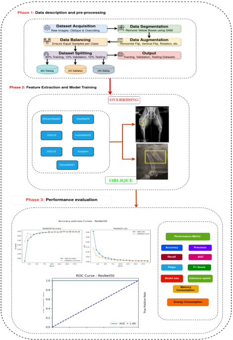
This study introduces a proposed model for classifying dog fractures using multiple pretrained models such as ResNet50, VGG16, VGG19, EfficientNetB0, Xception, MobileNetV2, and DesNet121. The proposed model consists of three phases as shown in Figure 1. These phases are explained in detail in the following sections.

Phase 1: Data description and preprocessing
The canine long bone fracture image dataset consists of 44 self-collected images (15 for oblique and 29 for overlay) from various sources, including Wikipedia (images of canine long bone fractures) as well as the Lawndale Veterinary Hospital website and the Billings Veterinary Clinic website.19, 20, 21. Figure 2 shows a sample of this dataset.

Selected samples from the canine long bone fracture dataset.
Data segmentation
We implemented a rigorous step of data segmentation preprocessing to ensure optimal input quality in the next classification phase. Specifically, we focused on the area within the yellow box in the data file. This region consistently included the main areas of fractures in the dogs studied. By segmenting and isolating this region, we attempted to improve the performance of the proposed DL by directing attention to the most relevant anatomical features and minimizing the influence of irrelevant underlying information. For this purpose, we used the Segment Anything Model (SAM), a modern segmentation algorithm developed by .twenty oneThis allowed us to accurately define the fractures within the yellow box, increasing the accuracy and generalization of the model.
The SAM algorithm accurately identified the yellow box by creating a segmentation mask and separating the features from the associated image information. This strategy improved data clarity and helped the classification model focus on important features during training, reducing the risk of unstable correlations and distortions.
Data segmentation has essentially proven to be a critical step in maintaining the integrity of the underlying visual information while at the same time effectively eliminating unnecessary components. This resulted in a cleaner and more refined dataset, clearly making it more suitable for downstream tasks such as element extraction, and ultimately for robust and reliable classification. Figure 3 visually illustrates the impact of segmentation on the dataset, clearly demonstrating the improvement in image quality by removing irrelevant elements and focusing on relevant visual information.

Sample dataset before and after segmentation.
Data augmentation
One of the key challenges in training ML models is ensuring that the dataset is large enough to enable accurate and generalizable predictions. In our case, the initial data file was relatively small, with only 29 images in the dominant class and 15 images in the oblique class. This limited number of samples reduces the model’s ability to learn a robust function, which can lead to suboptimal performance and reduced accuracy. To overcome this limitation, we used data augmentation techniques to expand the dataset and improve the model training process.twenty two.
The main purpose of data augmentation in our methodology was to increase the number of training samples and allow the model to learn more diverse and representative functions. By generating other variations of existing images, we focused on improving the model’s ability to generalize to unseen data and increase overall predictive accuracy. To achieve this, we used the keraras Imagedatagener algorithm. In this configuration, we used a number of transformations to create a varied and realistic sample while preserving the main visual elements.
-
Rotation: Images were randomly rotated by up to 40 degrees to simulate changes in orientation.
-
Zoom: A random zoom within a range of 20% was used to simulate changes in scale and distance.
-
Filling mode: New pixels introduced during transformation were filled with a constant value to maintain background consistency.
Through this process, the dataset was significantly expanded as shown in Figure 4.
-
The Overriding class has increased from 29 images to 2,843 images.
-
Oblique class increased from 15 images to 1446 images.

Dataset before and after expansion.
Balancing the data
The effectiveness of machine learning models is highly dependent on the balance of the training data.twenty three. Figure 5 shows the distribution of samples in the dog bone fracture dataset before and after using the data balance technique. Initially, there was a huge imbalance between the two classes. The oblique class consisted of 1,446 samples, while the dominant class contained 2,843 samples. Although the difference between the two classes was relatively small, even small imbalances can cause challenges during training.
-
Bias towards the majority class: A model trained on an unbalanced dataset may favor the majority class and ignore the minority class, resulting in suboptimal results.
-
Poor generalization: Imbalanced data can lead to overfitting, where the model does not generalize well to unseen data, especially underrepresented categories.
To solve these problems and ensure fair representation, we introduced a data balancing strategy using data augmentation. Specifically, I used the algorithm keras Imagedatagenerator. In this configuration, we used a number of geometric and photometric transformations to generate the other samples of the minority class (diagonal) so that both classes had the same number of samples. After balancing, each class contained 4,240 samples, eliminating the difference between the two categories.
The augmentation process introduced realistic variations to the image while preserving the main visual features. We applied data augmentations to the training images, including random rotation (up to 40 degrees), shearing, and zooming (up to 20%). The newly created pixels were processed using constant fill mode to keep the background consistent.
Having equal sample sizes for both classes ensures that the model learns equally from each category, improving classification accuracy.

Dataset before and after balancing.
Splitting the dataset
To ensure a robust and reliable evaluation of model performance, the dataset was divided into three different subgroups: training, validation, and testing.twenty four. The data was split as follows:
-
80% for training: Used to train the model by iteratively adjusting parameters.
-
10% for validation: Used to tune hyperparameters and monitor model performance during training, which helps prevent overfitting.
-
10% for testing: Reserved for unbiased evaluation of a fully trained model to ensure that its performance generalizes well to unseen data.
The splitting strategy balances training data requirements with independent subsets for validation and testing. The training set provides meaningful expressions, validation plays a key role with nine fine-grained hyperparameters, and the test set evaluates the generalization of the model to new samples.
The model is trained using 80% of the training data to ensure a diverse sample set for robust learning. A 10% validation set monitored model progress without jeopardizing the integrity of the test set and ensured representative results.
Phase 2: Feature extraction and model training
In this phase, we adopted the ResNet50 architecture.twenty five From element extraction to model training. ResNet50 is a 50-layer deep convolutional neural network designed to solve the vanishing gradient problem through residual learning. The architecture is structured into multiple phases, each containing a convolutional layer, normalization and activation functions, followed by an increasing gradient flow.
The model shown in Figure 6 starts with an initial 7×7 convolutional layer with 64 filters and stride 2 to process an input image of size 224×224 and reduce it to 112×112. This is followed by a 2×2 max-pooling layer to further reduce the spatial dimension to 56×56.
The core of ResNet50 consists of four main residual stages, and each stage contains multiple residual blocks. Each block consists of three convolutions.
-
1.
1 × 1 convolution to reduce dimensionality,
-
2.
3 × 3 convolution for feature extraction,
-
3.
1 × 1 convolution to restore dimensionality.
These residual blocks allow the network to retain important gradient information and alleviate the vanishing gradient problem. The stages are:
-
Stage 1: Three residual blocks with (64, 64, 256) filters. Maintain a feature map size of 56 × 56.
-
Stage 2: Three residual blocks with (128, 128, 512) filters. The spatial size is reduced to 28 × 28.
-
Stage 3: Three residual blocks with (256, 256, 1024) filters. The spatial size is reduced to 14 × 14.
-
Stage 4: Three residual blocks with (512, 512, 2048) filters. Reduce the space size to 7 x 7.
Following the final convolution block, a 2 × 2 pooling layer samples the features further downstream before passing them to a fully connected layer with 1000 output neurons, typically used for classification tasks.
During training, the model is optimized using a backpropagation algorithm with adaptive optimization techniques such as Adam. Batch normalization ensures stable learning and residual connectivity improves convergence, making ResNet50 an ideal architecture for detailed extraction of elements in comprehensive image recognition tasks.
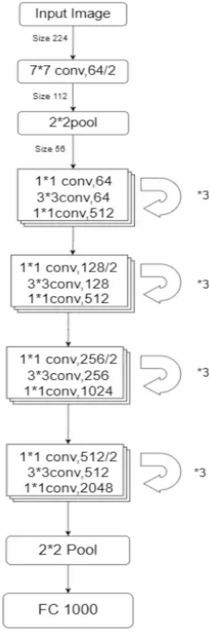
Proposed ResNet50 architecture.
Phase 3: Performance evaluation
The proposed ResNet5 model is evaluated for effectiveness and efficiency after training. Performance metrics are used to evaluate practicality in real-world scenarios, and accuracy is a key indicator of a model’s overall predictive performance.twenty two. Precision defined by Eq. (1) is the proportion of correctly predicted samples to the total predictions, indicating the overall predictive performance of the model.
$$\:Accuracy=(TP+TN)/(TP+TN+FP+FN)$$
(1)
Precision defined by Eq. (2) refers to the proportion of positive instances correctly predicted for a class compared to all positive predictions made for that class.
$$\:Accuracy=TP/(TP+FP)$$
(2)
Sensitivity, or recall, is the proportion of actual positive samples that are correctly recognized as positive according to Equation 1. (3).
$$\:Sensitivity\vee\:Recall=TP/(TP+FN)$$
(3)
The singularity expressed by Eq. (4) quantifies the proportion of negative samples that are accurately detected.
$$\:Singularity=TN/(TN+FP)$$
(4)
The F1 score is calculated by the weighted average of precision and recall, as shown in Equation 1. (5).
$$\:F1score=2\times\:\left(\right(precision\times\:recall)/(precision+recall\left)\right)$$
(5)
Here, FP stands for false positive and FN stands for false negative.


