This study utilized the integration of AI and AR in a smart photography classroom. Data were collected through the use of instructional videos demonstrating the photo creation process, based on which students were evaluated through performance measurements, surveys, and performance observations. For data processing, saliency-based filtering was utilized to improve image quality before applying a DRNN model using TensorFlow. AR apps support and enable interactive learning. This method showed the potential to increase student participation, enhance creativity and image analysis skills, and lead to improved educational outcomes in the field of photography and art. Figure 2 shows a workflow demonstrating the implementation of AI and AR techniques to enhance learning in a smart classroom environment.

AI-AR smart classroom learning enhancement flow proposal.
Augmented Reality (AR) Basics
AR is frequently used in smart classrooms to provide more engaging educational opportunities for students. AR provides consumers with novel and engaging ways to interact with content by superimposing computer-generated imagery (CGI) onto the user’s real-world environment. Tablets, smartphones, smartboards, and various applications all fall into the category of smart class extended display devices.
Designing Augmented Reality Instructional Videos
AR incorporates a wide range of technical components from multiple domains and disciplines as a holistic technology. The three-dimensional computer-generated virtual world or space produced by system simulation exists inside a computer. Through engagement, people may experience a virtual world or environment, giving the impression that they are actually there, due to the realistic sensory input it provides. According to some scholars, AR is a type of advanced human-computer interface that allows individuals to engage with their surroundings and communicate effectively in a three-dimensional virtual world. Based on this defined division, Figure 3 shows a specific division of the functional needs of an AR device into three systems.

For engagement, feedback, and real-time information sharing, it helped users perfectly simulate three-dimensional reality through a behavioral, perceptual, and computational measurement system for actions and operations. Data simulation is used to develop simulation systems through representational systems that provide commands for action and behavior, user engagement, information transfer to the user, and feedback to the user.
data collection
Smart Classroom learning data was collected from the open source kaggle. This dataset records 1,020 rows of learning outcomes, student innovation, and engagement in an intelligent classroom environment. The data will reflect performance measures such as visual literacy, aesthetic understanding, and engagement with augmented reality applications during photographic art workshops. Salience scores, session lengths, and final grades are all included.
Source: (https://www.kaggle.com/datasets/programmer3/smartclassroom-ai-ar-photography-insights).
Data preprocessing using saliency-based image filtering
Preprocessing is the first step in data analysis, converting raw data into a clean format that can be used for subsequent processing. Saliency-based image filtering is a preprocessing mechanism that focuses on preserving visually important concepts through the analysis of features such as contrast, color, and spatial location within an image. Equation (1) shows that the filtering step can improve important details while reducing noise and computation through visual learning tasks.
$$\begin{aligned} {V}_{j} & =\sum_{i=1}^{M}\Vert {d}_{j}-{d}_{i}\Vert { }^{2}{x}_{ji}^{\left(u\right)}\\ & ={D}_{j}^{2}\sum_{i=1}^{M}{x}_{ji}^{(u)}-{D}_{j}^{2}\sum_{i=1}^{M}{{d}_{i}x}_{ji}^{(u)}+\sum_{i=1}^{M}{{d}_{i}^{2}x}_{ji}^{(u)} \end{Align}$$
(1)
This equation calculates an informed weighted variance. \({V}_{j}\). is based on the distance between pixel values \({d}_{j}-{d}_{i}\) saliency weight \({x}_{ji}^{\left(u\right)}\)represents visual significance. In the preprocessing component of the study, this method filters out unfruitful image data by identifying salient regions. Through this method, AI-AR integration improves the recognition of meaningful compositions in the analysis of photo learning in smart classrooms.
Deep Recurrent Neural Network (DRNN)
Deep recurrent neural network (DRNN) algorithms are employed for intelligent image synthesis and feedback, enabling real-time analysis of composition and enhanced visual storytelling. DRNN is very suitable because it is effective in handling time series problems. DRNNs are effectively used for parameter projection in many applications including prediction, image processing, and many industries. The output response is evaluated using a cycle of feedback that includes the hidden output of the current instance and the embedded output of the previous instance. The feedback loop of the previous phase records data and uses both the immediate and intermediate outputs of the previous step to predict the final production. Figure 4 shows the basic structure of DRNN.

The computation is performed using the DRNN algorithm using the input series at time t. \((w = w1 \dots {w}_{j})\)hidden vector series \((g = g1, \dots {g}_{j})\)and the output vector I agree. The formula for this series is shown below. Equations (2 to 5) show the forward propagation equations that use the input characteristics, recurrent connections, and bias coefficients to calculate the activations of the DRNN.
$${net}_{i}=\sum_{i}{x}_{j,i}{w}_{j}+{x}_{gg}{g}_{j-1}+{\theta }_{j,i}$$
(2)
$${P}_{i}=e\left({net}_{i}\right)$$
(3)
$${net}_{l}=\sum_{l}{X}_{j,i}{P}_{i}+{\theta }_{i,l}$$
(4)
$${P}_{l}=e\left({net}_{l}\right)$$
(5)
where \({net}_{i}\) Shows the weighted average of the input layer and hidden layer. \({x}_{j,i}{w}_{j}\) represents the weight of the buried layer \({P}_{i}\) For subsequent time steps, and \(e\left({net}_{i}\right)\) The ratio of the importance of the hidden layer to the output layer. of \({\theta }_{i,l}\) Show the results of the hidden layer and output layer respectively. Equation (6) shows the sigmoid activation function used to determine the output probability of the DRNN model.
$$e\left(net\right)=\frac{1}{{1+e}^{(-net)}}$$
(6)
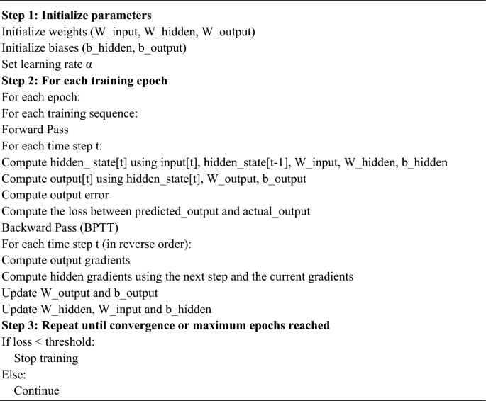
Real-time recursive learning (RTRL) and backpropagation in time (BPTT) are two training techniques that can be used to train a DRNN. Specifically, BPTT switches network parameters from a feedback to a feedforward architecture. A BPTT approach is used for this study, which consists of two main stages: forward pass and backward pass. In contrast, backward pass techniques calculate the mistakes and send the data from the output layer to the hidden layer. The following formula approximates the output layer error. Equation (7) shows the error function that describes the difference between the expected and actual output of the DRNN model.
$${f}_{l}={S}_{l}-{P}_{l}$$
(7)
Here, DRNN-based smart classroom system, \({S}_{l}\) represents the error function. \({S}_{l}\) is the ground truth saliency score, \({P}_{l}\) This is a prediction. This error is used to tell the network how to improve image-based artistic feedback for photography education. Equation (8), which is the derivative of the activation function of the DRNN, is used to calculate the slope of the loss with respect to the net input of the output layer.
$${\partial }_{l}={f}_{l}{\prime}e({net}_{l})$$
(8)
The smart classroom in the DRNN-based model incorporates photographic art. part of the equation \({\part }_{l}\) Define the local gradient as the derivative of the activation function \({f}_{l}\) Multiply errors in layers \({f}_{l}{\prime}e({net}_{l})\). This is used to propagate backwards in a timely and intelligent manner to generate images and feedback. In Equation (9), the DRNN training process uses the backpropagation error from the output layer and its derivative of the stimulus to calculate the gradient of the hidden layer node.
$${\partial }_{i}=e{\prime}({net}_{i}){\partial }_{l}{x}_{i,l}$$
(9)
equation \({net}_{i}\) Compute the backpropagation error in the neuron \(I\) In the context of DRNN-driven smart classrooms. \(e{\prime}({net}_{i})\) For photographic art, \({\part }_{l}{x}_{i,l}\) Connection weight. This helps optimize models to provide personalized creative feedback and image-based learning. Equations (10-12) show that the learning rate, error gradient, and prior activation are used in the weight and gate update equations of the DRNN model to maximize learning in smart classroom image synthesis.
$${\Delta x}_{i,l}=\alpha {\partial }_{l}{P}_{i}$$
(10)
$${x}_{i,l}={\delta x}_{i,l}+{\delta x}_{i,l}$$
(11)
$${\Delta x}_{gg}=\alpha {\partial }_{i}{g}_{j-1}$$
(12)
The weight update method during training is described by an equation using DRNN for smart classroom photo art. Based on the learning rate, \({\delta x}_{i,l}\) Change the weight. Weights are further refined \({\delta x}_{gg}\) and error gradient \(\alpha {\partial }_{i}{g}_{j-1}\) Power visual learning predictions and customized feedback. Equations (13–15) maximize feature learning in smart classroom settings and update the DRNN’s rules regarding iterative connections and input weights using gradient-based modifications.
$${x}_{gg}={x}_{gg}+{\delta x}_{gg}$$
(13)
$${\Delta x}_{j,i}=\alpha {\partial }_{i}{w}_{j}$$
(14)
$${x}_{j,i}={x}_{j,i}+{\delta x}_{j,i}$$
(15)
The iterative weight updates in these equations are consistent, which is intended to improve the teaching of photographic art using DRNN. meanwhile \({x}_{gg}+{\delta x}_{gg}\) Formula to change the weight between layers \(\alpha {\partial }_{i}{w}_{j}\) Update the weights iteratively using the gradient. Equations (16-19) show modifications that maximize the network’s learning accuracy for image-dependent materials.
$${\Delta \theta }_{i,l}=\alpha {\partial }_{l}$$
(16)
$${\theta }_{i,l}={\theta }_{i,l}+{\Delta \theta }_{i,l}$$
(17)
$${\Delta \theta }_{j,i}=\alpha {\partial }_{i}$$
(18)
$${\theta }_{j,i}={\theta }_{j,i}+{\Delta \theta }_{j,i}$$
(19)
Official use \({\delta \theta }_{i,l}\). The gradient-based update of weights across layers is represented by the following equation: \({\delta \theta }_{j, i}\). This facilitates the model to efficiently learn artistic features from preprocessed image data. The DRNN based on the BPTT algorithm is shown in Algorithm 1.
Setting parameters
Hyperparameters of DRNN method shown in Table 1