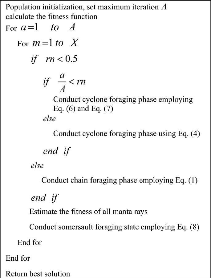
Conventional algorithm: MRFO
Numerous real-world optimization issues are relatively becoming difficult. Meta-heuristic approaches for managing the complexity of optimization issues are highly becoming famous. One of the nature-motivated optimization mechanisms is MRFO14, which offers a different optimization strategy for rectifying real-world optimization limitations. The intelligence of manta rays is considered in the existing MRFO. The manta rays have special foraging properties to resolve diverse optimization limitations. The MRFO’s functionalities are given as mathematically here.
The foraging properties including “chain foraging, cyclone foraging, and somersault foraging” are considered in this strategy.
“Chain foraging” The manta rays are capable to monitor the plankton’s regions and going towards them. The plankton’s concentration decides the particular region’s effectiveness. Automatically, the MRFO takes the best outcome obtained so far. This phase is expressed in Eqs. (1) and (2).
$$l_{m}^{p} \left( {a + 1} \right) = \left\{ {\begin{array}{*{20}l} {l_{m}^{p} \left( a \right) + j\cdot \left( {l_{bt}^{p} \left( a \right) – l_{m}^{p} \left( a \right)} \right) + \alpha \cdot \left( {l_{bt}^{p} \left( a \right) – l_{m}^{p} \left( a \right)} \right)} &\quad {m = 1} \\ {l_{m}^{p} \left( a \right) + j\cdot \left( {l_{m – 1}^{p} \left( a \right) – l_{m}^{p} \left( a \right)} \right) + \alpha \cdot \left( {l_{bt}^{p} \left( a \right) – l_{m}^{p} \left( a \right)} \right)} & \quad {m = 2,\ldots ,X} \\ \end{array} } \right.$$
(1)
$$\alpha = 2\cdot j\cdot \sqrt {\left| {\log \left( j \right)} \right|}$$
(2)
In this, the weight coefficient is defined by α and the mth manta ray’s region at a time a is specified by \(l_{m}^{p} \left( a \right)\) in pth dimension. The highly concentrated plankton is taken as \(l_{bt}^{p} \left( a \right)\) and the random vector is taken as j in the limit of 0 and 1.
“Cyclone foraging” If the plankton is found underwater, the manta rays swim toward it in a spiral form. The groups of manta rays are designing spirals to conduct the foraging. The cyclone foraging is expressed in Eq. (3) for the 2D space.
$$\left\{ {\begin{array}{*{20}l} {L_{m} \left( {a + 1} \right) = L_{bt} + j\cdot \left( {L_{m – 1} \left( a \right) – L_{m} \left( a \right)} \right) + e^{xc} \cdot \cos \left( {2\pi c} \right)\cdot \left( {L_{bt} – L_{m} \left( a \right)} \right)} \\ {K_{m} \left( {a + 1} \right) = K_{bt} + j\cdot \left( {K_{m – 1} \left( a \right) – K_{m} \left( a \right)} \right) + e^{xc} \cdot \sin \left( {2\pi c} \right)\cdot \left( {K_{bt} – K_{m} \left( a \right)} \right)} \\ \end{array} } \right.$$
(3)
In this, in the boundary of 0 and 1, the selected arbitrary variable is taken as c.
The motion property is enlarged to the n-D space and it is simply shown in Eqs. (4) and (5).
$$l_{m}^{p} \left( {a + 1} \right) = \left\{ {\begin{array}{*{20}l} {l_{bt}^{p} \left( a \right) + j\cdot \left( {l_{bt}^{p} \left( a \right) – l_{m}^{p} \left( a \right)} \right) + \beta \cdot \left( {l_{bt}^{p} \left( a \right) – l_{m}^{p} \left( a \right)} \right)} &\quad {m = 1} \\ {l_{bt}^{p} \left( a \right) + j\cdot \left( {l_{m – 1}^{p} \left( a \right) – l_{m}^{p} \left( a \right)} \right) + \beta \cdot \left( {l_{bt}^{p} \left( a \right) – l_{m}^{p} \left( a \right)} \right)} &\quad {m = 2,\ldots ,X} \\ \end{array} } \right.$$
(4)
$$\beta = 2e^{{j_{1} \frac{A – a + 1}{A}}} \cdot \sin \left( {2\pi j_{1} } \right)$$
(5)
In this, the highest iteration is declared by A and the weight coefficient is indicated by β. The selected arbitrary factor in the range of 0 and 1 is shown as \(j_{1}\).
Entire manta rays searching for food sources as its reference region, therefore the cyclone foraging stage attained good exploitation. This strategy enables the MRFO task to gain an effective global search and it is given in Eqs. (6) and (7).
$$l_{rn}^{p} = g^{p} + j\cdot \left( {d^{p} – g^{p} } \right)$$
(6)
$$l_{m}^{p} \left( {a + 1} \right) = \left\{ {\begin{array}{*{20}l} {l_{rn}^{p} \left( a \right) + j\cdot \left( {l_{rn}^{p} \left( a \right) – l_{m}^{p} \left( a \right)} \right) + \beta \cdot \left( {l_{rn}^{p} \left( a \right) – l_{m}^{p} \left( a \right)} \right)} &\quad {m = 1} \\ {l_{rn}^{p} \left( a \right) + j\cdot \left( {l_{m – 1}^{p} \left( a \right) – l_{m}^{p} \left( a \right)} \right) + \beta \cdot \left( {l_{rn}^{p} \left( a \right) – l_{m}^{p} \left( a \right)} \right)} &\quad {m = 2,\ldots ,X} \\ \end{array} } \right.$$
(7)
In this, the arbitrary boundary generated arbitrarily in the search area is taken as \(l_{rn}^{p}\) and for the pth dimension’s upper bound is given by \(d^{p}\). For the pth dimension’s lower bound is declared by \(g^{p}\).
Somersault foraging Here, the food’s area is referred to as a pivot. All manta rays swim front and back near the pivot. Hence, the region is updated. This strategy is derived in Eq. (8).
$$l_{m}^{p} \left( {a + 1} \right) = l_{m}^{p} \left( a \right) + Z\cdot \left( {j_{2} \cdot l_{bt}^{p} – j_{3} \cdot l_{m}^{p} \left( a \right)} \right),\quad m = 1,\ldots ,X$$
(8)
In this, the attribute of somersault is declared as \(Z\). It controls the manta ray’s somersault limit. Further, the two arbitrary factors in the range of 0 and 1 are taken as j2 and j3. Algorithm 1 elucidates the pseudo-code for MRFO.
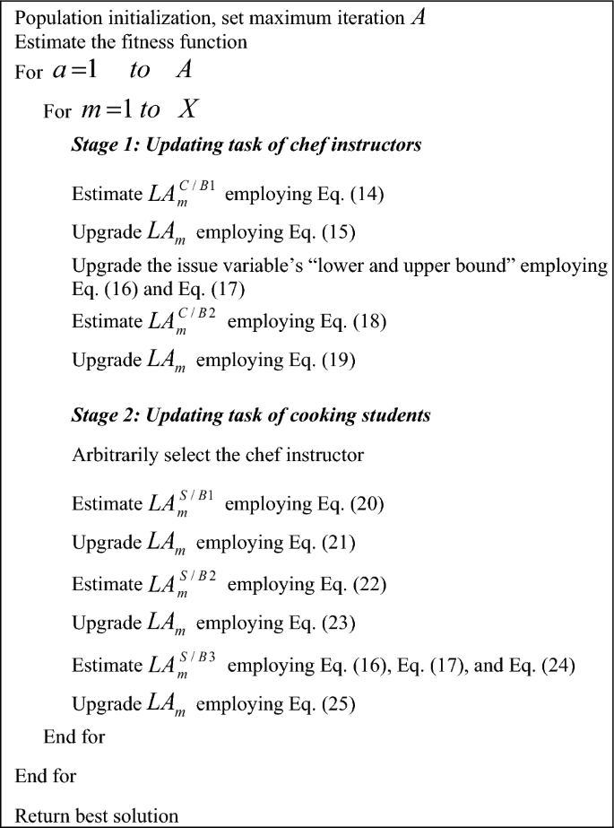
Conventional algorithm: CBOA
The CBOA15 is another meta-heuristic approach by inspiring the strategy of learning the cooking expertise in the training classes. The young and the cooking students are involved in the training classes to improve their cooking expertise and become chefs. This is employed in the CBOA concept.
Initialization The CBOA’s candidates are partitioned into two groups “chef instructors and cooking students”. The candidates of CBOA are shown in a matrix based on Eq. (9).
$$L = \left[ {\begin{array}{*{20}c} {L_{1} } \\ \vdots \\ {L_{m} } \\ \vdots \\ {L_{X} } \\ \end{array} } \right]_{X \times v} = \left[ {\begin{array}{*{20}c} {l_{1,1} } &\quad \cdots &\quad {l_{1,s} } &\quad \cdots &\quad {l_{1,v} } \\ \vdots &\quad \ddots &\quad \vdots &\quad {\mathinner{\mkern2mu\raise1pt\hbox{.}\mkern2mu \raise4pt\hbox{.}\mkern2mu\raise7pt\hbox{.}\mkern1mu}} &\quad \vdots \\ {l_{m,1} } &\quad \cdots &\quad {l_{m,s} } &\quad \cdots & \quad {l_{m,v} } \\ \vdots &\quad \ddots &\quad \vdots & \quad {\mathinner{\mkern2mu\raise1pt\hbox{.}\mkern2mu \raise4pt\hbox{.}\mkern2mu\raise7pt\hbox{.}\mkern1mu}} &\quad \vdots \\ {l_{X,1} } &\quad \cdots &\quad {l_{X,s} } &\quad \cdots &\quad {l_{X,v} } \\ \end{array} } \right]_{X \times v}$$
(9)
The population matrix is specified as L. The mth candidate of CBOA is denoted as \(L_{m}\) and its sth dimension is \(l_{m,s}\). The size of the population and the issue factor’s count for the objective function are X and s.
At first, the CBOA’s region is arbitrarily initialized employing Eq. (10).
$$l_{m,s} = g_{s} + j\cdot \left( {d_{s} – g_{s} } \right)$$
(10)
Here, for the sth issue factor’s upper bound is declared by \(d_{s}\). For the sth issue factor’s lower bound is declared by \(g_{s}\). The chosen arbitrary variable among 0 and 1 is specified as j.
In CBOA, the objective function is evaluated for each member employing Eq. (11).
$$Q = \left[ {\begin{array}{*{20}c} {Q_{1} } \\ \vdots \\ {Q_{m} } \\ \vdots \\ {Q_{X} } \\ \end{array} } \right]_{X \times 1} = \left[ {\begin{array}{*{20}c} {Q\left( {L_{1} } \right)} \\ \vdots \\ {Q\left( {L_{m} } \right)} \\ \vdots \\ {Q\left( {L_{X} } \right)} \\ \end{array} } \right]_{X \times 1}$$
(11)
In this, the fitness function’s vector is denoted as Q, and the mth member’s fitness function is specified as \(Q_{m}\).
After initialization, the CBOA moves to enhance the member outcome. The updating task of each group (chef and cooking student) is distinct. The arranged population matrix and fitness function are given in Eqs. (12) and (13).
$$LA = \left[ {\begin{array}{*{20}c} {LA_{1} } \\ \vdots \\ {LA_{NC} } \\ {LA_{NC + 1} } \\ \vdots \\ {LS_{X} } \\ \end{array} } \right]_{X \times v} = \left[ {\begin{array}{*{20}c} {la_{1,1} } &\quad \cdots &\quad {la_{1,s} } &\quad \cdots &\quad {la_{1,v} } \\ \vdots &\quad \ddots &\quad \vdots &\quad {\mathinner{\mkern2mu\raise1pt\hbox{.}\mkern2mu \raise4pt\hbox{.}\mkern2mu\raise7pt\hbox{.}\mkern1mu}} &\quad \vdots \\ {la_{NC,1} } &\quad \cdots &\quad {la_{NC,s} } &\quad \cdots &\quad {la_{NC,v} } \\ {la_{NC + 1,1} } &\quad \cdots &\quad {la_{NC + 1,s} } &\quad \cdots &\quad {la_{NC + 1,v} } \\ \vdots &\quad \ddots &\quad \vdots &\quad {\mathinner{\mkern2mu\raise1pt\hbox{.}\mkern2mu \raise4pt\hbox{.}\mkern2mu\raise7pt\hbox{.}\mkern1mu}} &\quad \vdots \\ {la_{X,1} } &\quad \cdots &\quad {la_{X,s} } &\quad \cdots &\quad {la_{X,v} } \\ \end{array} } \right]_{X \times v}$$
(12)
$$QA = \left[ {\begin{array}{*{20}c} {QA_{1} } \\ \vdots \\ {QA_{NC} } \\ {QA_{NC + 1} } \\ \vdots \\ {qS_{X} } \\ \end{array} } \right]_{X \times v}$$
(13)
Here, the chief instructor’s count is given as NC and the arranged CBOA’s population matrix is LA. The ordered objective function is QA. In the matrix LA, the candidates from \(LA_{1}\) to \(LA_{NC}\) define the chef instructors, whereas the candidates from \(LA_{NC + 1}\) to \(LA_{X}\) define the cooking students.
Updating the chef instructor group The chef instructors are highly accountable for instructing the cooking skills to the students who exist in school. In this mechanism, the best instructor is selected and tries to teach the technique to the instructor. According to this, the chef instructor’s region is upgraded by employing Eq. (14).
$$la_{m,s}^{C/B1} = la_{m,s} + j\cdot \left( {H_{s} – M\cdot ls_{m,s} } \right)$$
(14)
Here, the newly validated status of the arranged mth candidate is \(la_{m}^{C/B1}\) on the basis of the initial mechanism \(C/B1\) and its sth dimension is \(la_{m,s}^{C/B1}\). The better instructor is provided as H and its sth dimension is \(H_{s}\). From the set {1, 2}, the selected arbitrary variable is M. The updated region is accepted only if the fitness value is enhanced. It is derived in Eq. (15).
$$LA_{m} = \left\{ {\begin{array}{*{20}l} {LA_{m}^{C/B1} ,} &\quad {QA_{m}^{C/B1} < Q_{m} ;} \\ {LA_{m} } &\quad {else,} \\ \end{array} } \right.$$
(15)
Here, the \(LA_{m}^{C/B1}\) candidate’s fitness function is taken as \(QA_{m}^{C/B1}\).
In the next mechanism, the instructor concentrates to enhance her/his cooking skills on the basis of independent activities. Based on this strategy, for each instructor in the search region, an arbitrary region is produced employing Eqs. (16) to (18). If the arbitrary region enhances the fitness function, it is applicable for position updating employing Eq. (19)
$$g_{s}^{lcl} = \frac{{g_{s} }}{a}$$
(16)
$$d_{s}^{lcl} = \frac{{d_{s} }}{a}$$
(17)
$$la_{m,s}^{C/B2} = la_{m,s} + g_{s}^{lcl} + j\cdot \left( {d_{s}^{lcl} – g_{s}^{lcl} } \right),\quad m = 1,2,\ldots ,NC,\; j = 1,2,\ldots ,v$$
(18)
$$LA_{m} = \left\{ {\begin{array}{*{20}l} {LA_{m}^{C/B2} ,} &\quad {QA_{m}^{C/B2} < Q_{m} ;} \\ {LA_{m} } &\quad {else,} \\ \end{array} } \right.$$
(19)
Here, the issue factor’s “upper and lower” regions are given as \(d_{s}^{lcl}\) and \(g_{s}^{lcl}\). The iteration counter is indicated as a. Here, the newly validated status of the arranged mth candidate is \(la_{m}^{C/B2}\) on the basis of the initial mechanism \(C/B2\) and its sth dimension is \(la_{m,s}^{C/B2}\). Here, the \(LA_{m}^{C/B2}\) candidate’s fitness function is taken as \(QA_{m}^{C/B2}\).
Updating the cooking student’s group The students participated in the school to understand the skills of cooking and become chefs. Based on this mechanism, the student is arbitrarily selected in a class taught by the chef. This mechanism estimated the new region utilizing Eq. (20).
$$la_{m,s}^{S/B1} = la_{m,s} + j\cdot \left( {K_{{i_{m,s} }} – M\cdot la_{m,s} } \right)$$
(20)
Here, the newly validated status of the arranged mth candidate is \(la_{m}^{S/B1}\) on the basis of the initial mechanism \(S/B1\) and its sth dimension is \(la_{m,s}^{S/B1}\). The chosen chef instructor is provided as \(K_{{i_{m,s} }}\) by mth the student is \(H_{s}\). From the set {1, 2, …, NC}, the selected arbitrary variable is \(i_{m,s}\).
The updated region is exchanged for the existing region, it enhances the fitness function and it is designed using Eq. (21).
$$LA_{m} = \left\{ {\begin{array}{*{20}l} {LA_{m}^{S/B1} ,} &\quad {QA_{m}^{S/B1} < Q_{m} ;} \\ {LA_{m} } &\quad {else,} \\ \end{array} } \right.$$
(21)
Here, the \(LA_{m}^{S/B1}\) candidate’s fitness function is taken as \(QA_{m}^{S/B1}\).
In the second mechanism, each issue factor is considered to be a cooking expertise, and the student concentrates to learn any one chef instructor’s skill entirely. Based on this idea, a new region is estimated by employing Eq. (22).
$$la_{m,s}^{S/B2} = \left\{ {\begin{array}{*{20}l} {K_{{i_{m,s} }} ,} &\quad {s = n;} \\ {la_{m,s} ,} &\quad {else,} \\ \end{array} } \right.$$
(22)
Further, it is exchanged with the traditional region on the basis of Eq. (23), if it enhances the fitness function.
$$LA_{m} = \left\{ {\begin{array}{*{20}l} {LA_{m}^{S/B2} ,} &\quad {QA_{m}^{S/B2} < Q_{m} ;} \\ {LA_{m} } &\quad {else,} \\ \end{array} } \right.$$
(23)
Here, the newly validated status of the arranged mth candidate is \(la_{m}^{S/B2}\) on the basis of the initial mechanism \(S/B2\) and its sth dimension is \(la_{m,s}^{S/B2}\). Here, the \(LA_{m}^{S/B2}\) candidate’s fitness function is taken as \(QA_{m}^{S/B2}\).
In the third mechanism, each student concentrates to enhance his/her cooking skills on the basis of independent skills. Based on this idea, for each student in the search region, an arbitrary region is produced by Eqs. (16) and (17). Then, a new region is estimated by Eq. (24).
$$la_{m,s}^{S/B3} = \left\{ {\begin{array}{*{20}l} {la_{m,s} + g_{s}^{lcl} + j.\left( {d_{s}^{lcl} – g_{s}^{lcl} } \right),} &\quad {s = f;} \\ {la_{m,s} ,} &\quad {s \ne f,} \\ \end{array} } \right.$$
(24)
Here, the newly validated status of the arranged mth candidate is \(la_{m}^{S/B3}\) on the basis of the initial mechanism \(S/B3\) and its sth dimension is \(la_{m,s}^{S/B3}\). The variable f is selected from {1, 2, …, v}. Further, it is exchanged with the traditional region on the basis of Eq. (25), if it enhances the fitness function.
$$LA_{m} = \left\{ {\begin{array}{*{20}l} {LA_{m}^{S/B3} ,} &\quad {QA_{m}^{S/B3} < Q_{m} ;} \\ {LA_{m} } &\quad {else,} \\ \end{array} } \right.$$
(25)
Here, the \(LA_{m}^{S/B3}\) candidate’s fitness function is taken as \(QA_{m}^{S/B3}\). Algorithm 2 shows the pseudo-code of existing CBOA.
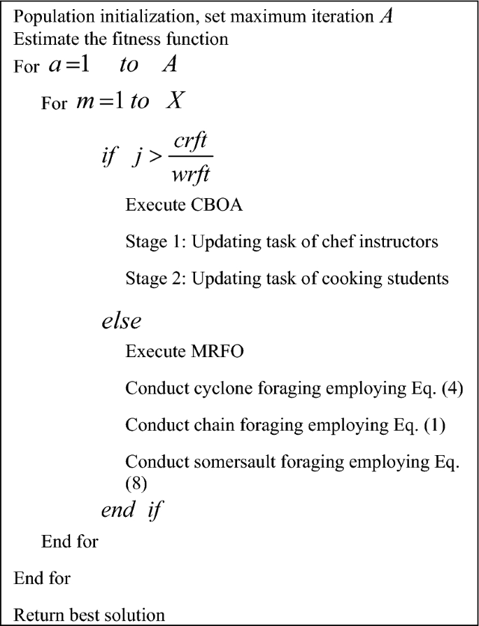
Proposed hybrid algorithm: HMRFO
The HMRFCO is implemented for optimizing the resource allocation, relay selection, and also the parameters such as steps per epoch, size of epoch, and the count of hidden neurons that exist in the ResGRU technique. Generally, resource allocation faces issues such as poor communication, and resource underutilization. Likewise, the relay selection has several limitations such as inference issues and higher energy consumption. In addition to that, though the deep learning techniques offer promising outcomes, it may face computational complexities. In order to prevent these problems, an effective optimization approach is necessary. Hence, the HMRFCO is introduced for this purpose.
The HMRFCO is the hybrid algorithm, where the CBOA and MRFO algorithms are integrated due to these algorithm’s improved performance rates. The CBOA provides better outcomes for optimization issues and dealing with real-time applications. Similarly, the MRFO can handle complex optimization issues and has better convergence values. However, the CBOA has lower convergence rates, and MRFO struggles to perform well in real time applications. Therefore, these two modern algorithms are integrated and supported in this work. The recommended HMRFCO works on the basis of fitness values and the arbitrary variable in the boundary of 0 and 1. The HMRFCO’s function is mathematically shown in Eq. (26).
$$\begin{aligned} &if\; \, j > \frac{crft}{{wrft}}\\ & \qquad \quad Update \quad CBOA \\ & else \\ &\qquad \quad Update \quad MRFO \\ \end{aligned}$$
(26)
Here, the random integer from the limit of 0 and 1 is pointed as j, and the worst fitness is declared as wrft. The current fitness is given as crft. If the selected random integer from 0 to 1 is greater than the value of \(\frac{crft}{{wrft}}\) is then the CBOA algorithm is executed or else the MRFO algorithm is executed. Thus, the HMRFCO is implemented for optimization purposes. The pseudo-code of the recommended HMRFCO approach is given in Algorithm 3 and Fig. 1 depicts the HMRFCO approach’s flowchart.

Flowchart of recommended HMRFCO approach for optimization purpose.