

Figure 1 illustrates the design and flowchart employed in this study:
-
1.
The physiological data obtained from MIMIC-IV was preprocessed.
-
2.
Four combinations of dynamic observation-prediction windows were defined.
-
3.
The dataset was divided into training and testing sets with an 8:2 ratio.
-
4.
Machine learning models were trained using all features and common features as inputs.
-
5.
The methods presented in this study were compared to two traditional metrics (ROX index, mROX index).
-
6.
Interpretability analysis and ablation experiments were performed using SHAP algorithm.

The study flowchart. Data from the MIMIC-IV database, with a total of 427 eligible patients was used. Among them, 393 instances of successful HFNC treatment and 105 instances of treatment failure were allocated into training and testing sets.
Source of data
The dataset utilized in this retrospective study was extracted by the MIMIC-IV database22. The MIMIC database was established in 2003 with funding from the National Institutes of Health (NIH) and is a collaborative effort involving the Laboratory for Computational Physiology at MIT, Beth Israel Deaconess Medical Center (BIDMC), and Philips Healthcare. Clinical data from over 190,000 patients and approximately 450,000 hospital admissions at BIDMC between 2008 and 2019 are included in the database. Demographic information, laboratory results, medication records, vital signs, surgical procedures, disease diagnoses, medication management, follow-up and survival status, and other detailed patient information is available.
Participants and eligibility criteria
AHRF is defined as the ratio of arterial partial pressure of oxygen (PaO2) to the fraction of inspired oxygen (FiO2) ≤ 300 mmHg6,23,24, and is not accompanied by hypercapnia23.
Although the 2023 ATS/ESICM criteria allow for the diagnosis of ARDS without the requirement for invasive mechanical ventilation, the absence of systematically recorded imaging findings (e.g., chest radiography or CT) and echocardiographic data to exclude cardiogenic pulmonary edema in the MIMIC-IV database precluded a definitive ARDS diagnosis. Therefore, we adopted the broader term acute hypoxemic respiratory failure (AHRF) defined as PaO2/FiO2 ≤ 300 mmHg without hypercapnia as a practical surrogate for cohort selection. This approach ensures consistency with the available data while still encompassing a large proportion of patients who likely fulfill the criteria for non-intubated ARDS25.
HFNC treatment success is defined as a downgrade of respiratory support to COT or spontaneous breathing after weaning from HFNC. HFNC treatment failure is defined as an upgrade of respiratory support to IMV or tracheostomy within one hour of weaning from HFNC.
In this study, various observation windows (1, 4, 8, and 12 h) were introduced to investigate the impact of observation duration on model performance in detail. Specifically, the 12-h window aligns with the recommended HFNC treatment duration26, where extending the observation period beyond 12 h may adversely affect early detection and timely intervention, increasing the risk of delayed intubation. Conversely, the 1-h window allows for more immediate prediction capability, while the 4-h and 8-h windows provide intermediate intervals between the shortest and longest durations, designed to explore how a gradual increase in window length affects model accuracy. These various observation windows not only balances the real-time responsiveness and accuracy of predictions but also aligns with clinical practices of evaluating HFNC efficacy, offering healthcare providers a range of decision-support options.
Observation window: The observation window was set to 1, 4, 8, and 12 h, respectively. The failure of HFNC treatment in patients with AHRF was predicted using the data within this window.
Prediction window: The prediction window was used to determine whether HFNC treatment failure occurred within this window period. Considering the demand for real-time prediction and clinical practice experience, a 4-h prediction window was used27,28.
Rationale for the window design: Clinically, the observation window reflects the period during which a physician would monitor patient vital signs and trends to form a clinical judgment, whereas the prediction window represents a realistic timeframe in which proactive interventions could be initiated if deterioration is anticipated.
Common features: physiological and clinical parameters obtained without requiring arterial catheterization, blood sampling, or other invasive procedures.
Figure 2 and (Appendix 1 (Supplementary Fig. 1)) shows the combination of a 1-h observation window and a 4-h prediction window as an example to illustrate the real-time dynamic warning window.

Implementation diagram of the dynamic window. The combination of set observation window and prediction window slides every hour along the timeline.
The following criteria were used to enroll patients into the study:
-
a.
Adult patients (age ≥ 18 years).
-
b.
Diagnosed with AHRF.
-
c.
Undergoing HFNC treatment.
-
d.
HFNC treatment duration between 12 and 48 h.
The detailed process of data selection is shown in Fig. 3.
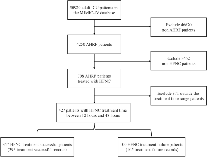
Process for selection of the cohort.
Based on the aforementioned four criteria, a total of 427 patients were included. There were 498 instances of HFNC treatment recorded, including 393 instances of successful treatment and 105 instances of treatment failure. Each recorded HFNC treatment instance in this study was treated as an independent sample for analysis.
Outcome definition and predictors
A total of 30 features were extracted from the MIMIC-IV database. The common features included demographic features, physiological features and Glasgow Coma Scale score. The laboratory features comprised blood gas analysis, chemistry assay, and complete blood cell count. The selection of these features was informed not only by our previous work and related studies on intubation prediction, but also by their clinical relevance in capturing the patient’s overall physiological status and oxygenation dynamics. Especially during HFNC treatment, these features dynamically capture changes in respiratory function and metabolic condition, providing critical inputs for the model to predict patients’ responses to treatment. The hourly median of numerical data was used, with a sampling frequency of 1 h. Table 1 presents the selected features and their types.
Data preprocessing and handling of missing data
Data standardization
Data standardization was performed using the Z-score method29. Z-score normalization was used to scale each feature to a standard normal distribution with a mean of zero and a standard deviation of one. This normalization method eliminates the scale differences between different features, making the feature weights more consistent and facilitating model convergence.
Missing value imputation
The following imputation methods were used for physiological features: For urine output, if the patient had a null value for a particular hour, it was assumed that there was no urine output during that hour, and thus it was imputed with zero. For other physiological features, the previous value was used for imputation. If there was no previous value, the global median was used instead.
One-hot encoding
One-hot encoding is a widely used technique often employed to convert categorical variables into a format suitable for machine learning methods. In one-hot encoding, each value of a categorical variable is transformed into a binary vector of length equal to the number of possible values of that variable. Only one element in the binary vector is set to 1, while the others are set to 030. The position corresponding to the specific value of a variable is marked as 1. In this study, one-hot encoding was used to process the gender variable.
Data imbalance issue
To address the issue of data imbalance, this study employed a “pseudo-over-sampling” method for data balancing. Specifically, for each patient, the number of virtual data rows equal to the length of the prediction window was added—in this study, 4 rows of virtual data were added for each patient. These 4 rows of data were identical to the last row of the patient’s real data. When the dynamic window slides to the maximum extent in the time series, the prediction window exactly occupies the 4 rows of virtual data, while the observation window slides to the last hour of the real data. The advantages of this method are as follows:
(1) The amount of positive data was increased, expanding the number of positive data rows by 4 times; (2) During model training, only the binary classification labels of the virtual data were used, without incorporating the virtual data itself into model training; (3) The observation window only included all real data.
Model development
In this study, five machine learning methods and a soft voting ensemble machine learning algorithm were employed, and the results were compared to the ROX and mROX indices. To further enhance the predictive performance of these models, a custom grid search method incorporating an optimal classification threshold algorithm was employed for hyperparameter optimization. Taking the LGBM algorithm as an example, the primary optimized hyperparameter settings are as follows: the number of trees (n_estimators), tree depth (max_depth), and number of leaves (num_leaves) are set to 100, 10, and 31, respectively.
Logistic regression (LR)31: A linear model used in binary classification problems by transforming the linear combination of input features into probability outputs using a logistic function.
Naive Bayes (NB)32: Based on Bayes’ theorem and the assumption of conditional independence between features, this model works well with high-dimensional data but performs poorly in the presence of feature dependencies.
Support vector machine (SVM)33: A supervised learning algorithm used for classification and regression tasks, which calculates an optimal hyperplane in a high-dimensional space to maximize the margins between categories, thus achieving data classification.
Random forest (RF)34: An ensemble learning model composed of multiple decision trees that improves the accuracy of classification or regression by using majority voting or the mean prediction of the individual decision trees for classification and regression, respectively.
LGBM (LightGBM)35: A decision tree algorithm based on the gradient boosting framework, which accelerates the training process using histogram-based algorithms, suitable for large-scale datasets.
Long Short-Term Memory (LSTM)36:A type of recurrent neural network (RNN) architecture designed to capture long-term dependencies in sequential data by using memory cells and gating mechanisms. It is particularly well-suited for modeling time-series data, such as physiological signals, where temporal dynamics play a crucial role in prediction tasks.
Soft voting ensemble machine learning algorithm37: The soft voting ensemble machine learning method is an ensemble learning technique that aggregates the probability predictions of multiple base models to make decisions, thereby improving classification or regression accuracy. Figure 4 illustrates the principle of the soft voting ensemble machine learning algorithm. In this study, three models (LR, RF, LGBM) with smaller differences in sensitivity and specificity and higher AUC values were used in the soft voting ensemble.
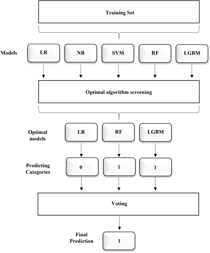
The principle of soft voting ensemble machine learning algorithms. LR Logistic regression, NB Naive Bayes, SVM Support vector machine, RF Random forest, LGBM LightGBM.
LR, NB, SVM, RF, LGBM, and LSTM represent classic algorithms in the fields of statistics, probability theory, geometry, decision tree modeling, gradient boosting, and deep learning, respectively. The soft voting ensemble machine learning algorithm enhances the performance and stability of the overall model by aggregating the prediction results of multiple base learners, so as to achieve more accurate and reliable predictions.
Model performance and validation
Traditional prediction methods
ROX Index: The ROX index threshold of 4.88 was adopted to predict HFNC treatment failure, whereby values below 4.88 were interpreted as likely treatment failure and values equal to or above 4.88 as likely treatment success. This threshold is broader than the commonly used cutoff of 3.85 reported in previous studies, and was intended to allow for a more inclusive identification of patients at high risk of treatment failure38,39.
mROX Index16: The mROX index is an improvement of the ROX index, where SpO2 is replaced with PO2 to more accurately reflect oxygenation status. Li16 evaluated the predictive effect of the mROX index at the 2nd hour after initiating HFNC. Therefore, in this study, an mROX index less than 4.3 at the 2nd hour after initiating HFNC was used to predict treatment failure, based upon previous research.
Performance evaluation metrics
The following metrics were used to evaluate the performance of the machine learning models: Accuracy (ACC), area under the curve (AUC) of the receiver operating characteristic (ROC) curve, sensitivity (SEN), specificity (SPE), Bayesian error rate (BER), Matthews correlation coefficient (MCC), F1-score, and KAPPA40. Table 2 presents the calculation formulas and brief descriptions of these eight metrics.
Internal validation
Temporal internal validation was performed by training the model on data from 2008 to 2013 and testing on data from 2014 to 2019, using a 1-h observation window and a 4-h prediction window.
Model explainability analysis
SHAP-based interpretation of feature contributions
To enhance interpretability, SHapley Additive exPlanations (SHAP) were applied to quantify the contribution of each predictor to the model output. SHAP values represent the marginal contribution of individual features to a given prediction, derived from cooperative game theory. This approach allows for both global interpretation by summarizing the average impact of features across the dataset and local interpretation, which reveals how specific features influence predictions for individual patients.
Feature selection using recursive elimination
Recursive feature elimination with cross-validation (RFECV) was performed to evaluate the trade-off between model complexity and predictive performance. This technique iteratively eliminated the least important features based on model performance metrics, resulting in a parsimonious subset of predictors. The selected features were subsequently used for final model development to optimize both performance and interpretability.
Calibration analysis for clinical reliability
Model calibration was assessed using the Brier score, which quantifies the mean squared difference between predicted probabilities and actual outcomes. Lower Brier scores indicate better calibration. Comparative calibration analysis across all candidate models demonstrated that the ensemble model consistently achieved the lowest Brier scores, suggesting a higher degree of reliability in predicted probabilities.
Software and reproducibility
All data preprocessing, feature selection, model training, and interpretability analyses were conducted using Python 3.12 in a Jupyter Notebook environment. The computational workflow was based on open-source packages including scikit-learn, LightGBM, SHAP, XGBoost, pandas, and NumPy. Model development and visualization were performed interactively in Jupyter Notebook. The source data were stored and queried from a PostgreSQL 15.3 database, which was used for efficient data extraction and time window alignment from the MIMIC-IV relational database.


