Predictive fault management in smart sensor networks using a dynamic quantum-AI architecture (DynaQuAI)

System architecture overview

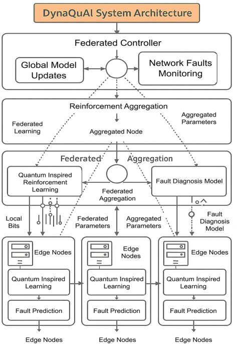
Figure 1 reflects the entire DynaQuAI framework. The framework can be described as the three layers, where all are linked: the edge sensor layer that houses heterogeneous sensors, which gather multimodal data; the local learning layer, which provides single nodes with quantum-inspired reinforcement learning, and allows fault diagnosis; and the federated aggregation layer, which provides collaborative model improvement through the synchronization of secure parameters.

Every sensor component consists of three operating modules. The local-state-representation module receives sensor streams that provide non-redundant, corresponding multimodal features—including temperature, vibration, power consumption, and signal quality metrics—and actively adjusts the feature space in response to network behavior through adaptive dimensionality reduction The quantum-inspired RL is a quantum bit-exploration based distributed learning control, which is implemented in the quantum-inspired RL module and does not store fault policies locally. Access to model parameters has been combined with privacy preserving protocols in the federated communication module making sure that sensitive data regarding operational activities does not leave individual nodes.

The federated aggregation controller coordinates the process of synchronizing the parameters within the network with adaptive scheduling taking into consideration heterogeneous communication capabilities. In place of the synchronous updates all nodes must engage in a constraint infeasible in sensor networks where nodes may often experience temporary connectivity loss the controller does asynchronous aggregation using straggler-sensitive algorithms that consider all received node updates and ensures convergence.

System model and problem formulation

We assume a mass wireless sensor network (WSN) that consists of \(\:N\) heterogeneous edge nodes that are spread over industrial and building scenarios. The multimodal sensors found in each node are temperature, vibration, power consumption, and radio signal quality sensors. Nodes are constrained in the resource allocation of low CPU frequency, limited memory and battery operated. The devices communicate using an IEEE 802.15.4 mesh network which is inherently intermittent in nature, loss and with variable link quality.

Network model

Let \(\:\mathcal{N}=\{1,2,\dots\:,N\}\) denote the set of edge nodes. Each node \(\:i\) collects a sensor observation vector

where \(\:M\) is the quantity of sensor modalities. A local VAE encoder is used to make a small representation of latent state.

which serves as the state input for the reinforcement learning (RL) policy. At each timestep, node \(\:i\) selects an action \(\:{a}_{i}\left(t\right)\) according to its local policy \(\:{\pi\:}_{{\theta\:}_{i}}\left(a|z\right)\) and receives a reward signal \(\:{r}_{i}\left(t\right)\) related to correct or incorrect fault decisions, energy consumption, and communication cost.

A federated server does asynchronous aggregation of local model parameters, which allows a global policy to be created without exchanging raw data. Masked and privacy preserving updates are only passed across.

Assumptions

In order to base the problem we assume the following practical assumptions:

• Edge nodes possess very little computational resources, storage and battery and the maximum possible CPU usage can be less than 5%.

• The connection through wireless is intermittent hence federated learning (FL) needs to be asynchronous.

• Finally, the raw sensor data are not transferred out of the node because of bandwidth and privacy reasons.

• The tags of faults are taken in historical logs or response logs through the Internet.

• The RW is partially observable as some variables of faults cannot be directly measured.

Optimization objective

DynaQuAI aims to study a global policy \(\:\pi\:\) that will reduce the overall cost of fault misclassification including the computation and communication overhead cost across the network:

where:

• \(\:{L}_{\text{fault}}\) penalizes incorrect or delayed fault detection,

• \(\:{E}_{\text{comp}}\) models local computation cost related to VAE and RL inference,

• \(\:{C}_{\text{comm}}\) represents communication overhead during FL parameter exchange,

• \(\:\lambda\:\) and \(\:\mu\:\) control the trade-off between accuracy, efficiency, and bandwidth usage.

Constraints

The optimization is operational and has typical edge deployment operational constraints:

This implementation defines a clear model of the system and a purpose, which offers a good basis to the quantum-inspired RL and federated learning systems offered in further sections.

Quantum-inspired reinforcement learning framework

Probabilistic state representation (quantum-inspired analogy)

We also develop sensor network fault diagnosis as a Markov decision process (MDP) whose state space is the current system state (corresponding to multimodal readings of sensors). Instead of traditional fixed state representations, probabilistic encoding of quantum states is proposed and inspired by quantum superposition: bitwise insurance planning is executed physically with quantum brightness (Tables 2 , 3, 4, 5).

We adopt a probabilistic encoding for sensor state representation, drawing a mathematical analogy with quantum bit (qubit) representations. For each sensor modality i ∈ {1, 2, …, M} where M represents the total number of sensor modalities, we define a two-component probability vector:

where \(\:{\alpha\:}_{i}\left(t\right)\) and \(\:{\beta\:}_{i}\left(t\right)\) represent complex probability amplitudes satisfying normalization constraint:

These quantum principles are then probabilistically represented in classical representations in our classical implementation. Each sensor modality \(\:i\) has a probability distribution over two representative features of the raw sensor measurements, with which efficient exploration is made possible without any direct quantum hardware resources, as well. The classical state is mapped to become like. Equation (4) uses Dirac bra-ket notation \(\left| \psi \right\rangle = {\text{ }}\alpha \left| 0 \right\rangle + {\text{ }}\beta \left| 1 \right\rangle\) as a mathematical analogy only. In implementation, this is simply a two-component probability vector.

\(\:\left(\begin{array}{c}{\left|{\alpha\:}_{i}\left(t\right)\right|}^{2}\\\:{\left|{\beta\:}_{i}\left(t\right)\right|}^{2}\end{array}\right)\:\) with the constraint p_i⁰ + p_i¹ = 1. No complex amplitudes, quantum gates, or quantum hardware are involved. The notation is retained for concise mathematical exposition while the computation is entirely classical

where \(\:{x}_{i}\left(t\right)+{y}_{i}\left(t\right)=1\) maintains the probability constraint. The composite system state combines all modalities:

Their diversity allows sensor modalities to be analyzed in terms of the interdependencies between them, and the dimensionality to be brought to an efficient manageable level with the use of powerful tools of caring it out in the form of a set of tensors. In cases where each of the modalities dimension \(\:{2}^{M}\). However, we employ tensor train decomposition to represent \(\:S\left(t\right)\) with computational complexity \(\:O\left(M{r}^{2}d\right)\) where \(\:r\) denotes the tensor train rank typically small in practice (3–5) and \(\:d\) is the maximum mode dimension.

Oscillatory exploration with probabilistic temperature scheduling (quantum-inspired analogy)

We generate a quantum-inspired exploration method which improves the original epsilon-greedy strategy by a probabilistic exploration similar to quantum superposition. Instead of choosing the action with probability e at random, we store a superposition-inflated probability distribution on the candidates of action by their expected event value.

The action value function \(\:Q\left(s,a\right)\) at state \(\:s\) with action \(\:a\) is estimated through neural network approximation \(\:{Q}_{\varphi\:}\left(s,a\right)\) with parameters \(\:\varphi\:\). Normalize the action likelihoods obtained using softmax be the values:

where \(\:\tau\:\) represents the exploration trade-off parameter. Our way of quantum inspirations brings in a dynamic scheduling of temperature according to quantum like phase rotations:

where \(\:{\tau\:}_{0}\) initializes the temperature, \(\:\lambda\:\) controls exponential decay, \(\:\omega\:\) represents the phase rotation frequency, and \(\:{\varphi\:}_{0}\) is an initialization phase. Clarification on ‘Quantum-Inspired’ Terminology: The cosine-squared temperature schedule in Eq. (9) produces periodic oscillations that are mathematically similar to quantum interference patterns but are computed using standard trigonometric functions on classical hardware. Throughout this paper,

• ‘Quantum-inspired’ refers exclusively to mathematical analogy:

• ‘Superposition-like’ means: classical probability distribution over actions via softmax (Eq. 8);

• ‘Interference patterns’ means: periodic cos²(ω_t + φ₀) modulation of exploration temperature;

• ‘Qubit encoding’ means: two-component probability vector per sensor modality (Eq. 6);

• ‘Amplitude perturbation’ means: stochastic action perturbation via XOR of random bits (Eq. 11).

No quantum computing, quantum gates, quantum circuits, or quantum hardware is required or used at any point in this framework. The square of the cosine makes periodic wave the waves are like quantum wave interference patterns that allow systematic search exploration that systematically revisits promising areas and gradually narrows down to exploitation.

In step \(\:e\) of the exploration phase, exploration intention is sampled by first sampling an action:

Then, with probability \(\:\gamma\:\left(t\right)={\gamma\:}_{0}{\left(1-\frac{t}{T}\right)}^{2}\) (where \(\:T\) is the total training horizon), we perturb the selected action through quantum-inspired amplitude perturbation:

where \(\:\oplus\:\) denotes action space addition, and \(\:{b}_{i}\) represent randomly sampled bits simulating quantum bit flips. The XOR combination has the effect of giving interference like patterns in the exploration trajectory similar to quantum wavefunction interference.

Value function learning with quantum principles

Temporal difference learning with quantum-inspired bootstrapping is used to estimate the value function \(\:V\left(s\right)\) representing the expected cumulative discounted reward in the state \(\:s\). The TD target takes into account the quantum inspired quantification of uncertainty:

where \(\:r\left(t\right)\) is the immediate reward, \(\:\gamma\:\in\:\left[0,1\right]\) is the discount factor, \(\:{V}_{\varphi\:{\prime\:}}\) represents the target network with parameters \(\:\varphi\:{\prime\:}\) updated periodically, and \(\:\delta\:\left(t\right)\) is the quantum-inspired uncertainty term:

The uncertainty term is proportional to the visitation frequency of the state \(\:{N}_{\text{visit}}\left({s}_{t+1}\right)\), which puts into practice optimism under the uncertainty principle which is central to exploration-exploitation theory. Uncertainty (high visitation) is stimulated by higher uncertainty and exploitation by confidence (high visitation). The scaling \(\:\sigma\:\left(t\right)={\sigma\:}_{0}\text{e}\text{x}\text{p}\left(-{\lambda\:}_{\sigma\:}t\right)\) can make the process of exploration gradual and allows an eventual shift towards exploitation.

The value function network has three layers: the input layer that takes state \(\:s\), hidden layer of dimension \(\:H\) that helps in feature extraction, and an output layer that predicts a scalar value. The value learning loss can be obtained as:

Similarly, the policy network \(\:{\pi\:}_{\theta\:}\left(a|s\right)\) with parameters \(\:\theta\:\) is learned through policy gradient with quantum-inspired advantage weighting:

where advantage function \(\:{A}^{Q}\left(s,a\right)={Q}_{\varphi\:}\left(s,a\right)-{V}_{\varphi\:}\left(s\right)\) is computed using learned state and action value functions. The quantum-inspired aspect brings about the effective difference in the weighting of benefits:

where controls the strength of modulation of the advantage and \(\overset{\lower0.5em\hbox{$\smash{\scriptscriptstyle\leftharpoonup}$}} {Q} \left( s \right) = {\mathbb{E}}_{a} Q_{{\varphi \:}} \left( {s,a} \right)\) is the mean of the actions. This weighting gives more weight to the areas around the mean (high uncertainty) but dampens far flanking advantages (high confidence areas) which is consistent with exploration principles of uncertainty quantification.

Elaboration on Quantum Inspiration: The investigation mechanism formulated in DynaQuAI is not similar to regular noisy or optimistic reinforcement methods in learning. In conventional noisy RL, additive stochastic noise is usually added directly to the Q-values or state logits, and optimistic approaches common in such systems reproduce the common artificially manipulated effect of adding higher values in states that are rarely visited. We instead encode state using amplitude rather than the binary state approach; and use a dynamic temperature scheduling that is based on a cosine-squared dynamics.

The encoding of qubits maps probability mass \(\:\left({\left|{\alpha\:}_{i}\left(t\right)\right|}^{2},{\left|{\beta\:}_{i}\left(t\right)\right|}^{2}\right)\) to the training of each sensor modality, which is not due to random noise but, like any other form of uncertainty, organized. These amplitudes vary the exploration distribution by altering both softmax policy of the inquiry in the Eq. (5) and the variation of temperature in Eq. (6). However, in contrast to monotonic decay in temperature of the classical RL, periodic cos \(\:{\text{c}\text{o}\text{s}}^{2}\left(\omega\:t+{\varphi\:}_{0}\right)\) has constructive interfering patterns and destructive interfering patterns like in the behavior of quantum waves. This makes the policy revisit the previously explored actions in a periodic manner even at advanced stages of training and therefore less chances exist of premature convergence.

Expository two-action conflict: An example is given of a simple case, two actions: \(\:A\) and \(\:B\). In classical softmax-based exploration, the probability of selection at time t is solely determined by the relative Q-values as well as over a set temperature constant or a decaying temperature. When \(\:Q\left(A\right)\) falls a little above \(\:Q\left(B\right)\) in the early stages of training, the policy will become attached to \(\:A\), which will decrease the possibility of exploration.

Conversely, DynaQuAI has amplitude weights \(\:\left({\left|\alpha\:\right|}^{2},{\left|\beta\:\right|}^{2}\right)\) which represent the uncertainty of each action. When there is uncertainty, these amplitudes cause both the actions to be put in a joint superposition-like position with neither action being suppressed. Even the temperature fluctuating term \(\:\tau\:\left(t\right)\) induces systematic expansion of the policy distribution:

working as imitation patterns. Consequently, the agent will automatically reconsider action \(\:B\) when it comes up even when \(\:Q\left(A\right)\) is temporarily in the lead. This behavior cannot be replicated under mere noise injection of Gaussian form, or simple optimistic initialization.

The combination of the amplitude-based encoding and temperature modulation through interference forms exploration patterns that are similar to quantum superposition and interference on classical hardware, which provide much more balanced and structured exploration of the policy space.

Federated learning with privacy preservation

Local model training

Local reinforcement learning policies are exposed to data generated in each sensor node to train the policies. The learners are interpolated with value functions and updates with a policy gradient, the final form of the local training objective:

where \(\:{L}_{\text{ent}}\left(\theta\:\right)=-\beta\:{\mathbb{E}}_{s,a}\left[{\pi\:}_{\theta\:}\left(a|s\right)\text{l}\text{o}\text{g}{\pi\:}_{\theta\:}\left(a|s\right)\right]\) represents entropy regularization encouraging exploration, and \(\:\lambda\:\), \(\:\beta\:\) are weighting coefficients. Entropy term does not allow the premature convergence of policy to deterministic solutions, instead, it keeps the exploration flexibility that is important to identify new fault patterns.

Each node \(\:n\) maintains local model parameters \(\:\left({\varphi\:}_{n},{\theta\:}_{n}\right)\) updated through SGD with batch size \(\:B\) and learning rate \(\:\eta\:\):

The local training operates concurrently leveraging unbroken sensor information and neglecting the dissemination of synchronous signals that allow deliberative reaction to local erroneous configurations and sustaining minimal delay.

Secure parameter aggregation

The sensor nodes transfer learned parameters to the federated aggregation controller where global model refinement is obtained periodically. Our privacy protection mechanisms involve use of the secure multi-party computation (SMPC) protocols that aggregate parameters and no node or a controller is able to see the contribution of any individual node.

The aggregation uses additive masking described by which each node \(\:n\) uses a random noise vector \(\in _{n}\) n to the parameters prior to transmission:

The masking noise \(\in _{n}\) is sampled from \({\mathcal{N}}\left( {0,\sigma \:_{ \in }^{2} I} \right)\). The aggregation controller is able to calculate: since masked parameters of all nodes add up to the actual aggregated parameters:

The zero-sum constraint in Eq. (20) requires all N nodes to submit masked parameters simultaneously. Under asynchronous aggregation, only a reporting subset S_r ⊆ {1, …, N} participates per round, with |S_r| ≤ N. When |S_r| < N, the global zero-sum property fails:

∑(n ∈ S_r) ε_n ≠ 0 (residual mask noise corrupts aggregation).

To resolve this, the global zero-sum masking is replaced with an asynchronous-compatible.

Pairwise privacy masking protocol:

Setup phase (one-time, before training):

Each pair of nodes (i, j), where i < j, agrees on a shared random seed s_ij via authenticated Diffie–Hellman key exchange over TLS 1.3. Each node i distributes its seed collection {s_ij : j ≠ i} using Shamir’s (t, N)-threshold secret sharing among all other nodes, where \(t = \left\lceil {2N/3} \right\rceil\).

Mask generation (each round r):

Each node i computes its aggregate privacy mask as:

where PRG(s, r) is a cryptographic pseudorandom generator keyed by seed s with round counter r. The masked parameter update transmitted by node i is:

$$\tilde{\varphi }_{i} ^{{\left( r \right)}} {\text{ }} = {\text{ }}\varphi _{i} ^{{\left( r \right)}} {\text{ }} + {\text{ }}m_{i} ^{{\left( r \right)}}$$

(23)

Pairwise cancellation property:

For any two nodes i, j both present in S_r, their mutual mask contributions cancel exactly: PRG(s_ij, r) − PRG(s_ij, r) = 0. The only residual comes from edges crossing the boundary of S_r:

$$\tilde{\varphi }_{i} ^{{\left( r \right)}} {\text{ }} = {\text{ }}\varphi _{i} ^{{\left( r \right)}} {\text{ }} + {\text{ }}m_{i} ^{{\left( r \right)}}$$

(24)

Dropout recovery:

For each dropped node j ∉ S_r, the aggregation server collects t Shamir shares from surviving nodes in S_r (requiring |S_r| ≥ t) to reconstruct j’s seeds {s_ij}. The server computes the residual mask contributions and recovers the exact aggregate:

$$\varphi ^{{\left( r \right)}} = {\text{ }}\left( {1/|S_{r} } \right){\text{ }}\sum (i \in S_{r} ){\text{ }}\varphi ^{{\left( r \right)}}$$

(25)

Theorem 1: Privacy under asynchronous aggregation

Under the pairwise masking scheme with (t, N)-threshold Shamir secret sharing, for any reporting subset S_r with |S_r| ≥ t:

1. (i)

   Correctness: The server recovers the exact weighted average (\(\left( {1/\left| {S_{r} } \right|} \right)\,\sum i \, \in \,S_{r} \,\varphi _{i} ^{{\left( r \right)}}\).

2. (ii)

   Privacy: The server learns no individual φ_i⁽ʳ⁾, provided at most (t − 1) nodes collude with it.

3. (iii)

   Dropout tolerance: Up to (N − t) nodes may drop out per round without affecting correctness.

Deployment note: For the 500-node deployment with t = 334, the system tolerates up to 166 simultaneous node dropouts per round while maintaining both correctness and privacy guarantees. Differential privacy is additionally achieved by calibrating noise injection on top of the pairwise masking.

The aggregated global model parameters \(\overset{\lower0.5em\hbox{$\smash{\scriptscriptstyle\leftharpoonup}$}} {\varphi }\), \(\overset{\lower0.5em\hbox{$\smash{\scriptscriptstyle\leftharpoonup}$}} {\theta }\) are then broadcast to all nodes:

$$\:\varphi \:_{n}^{{t + 1}} = \left( {1 – \rho \:} \right)\varphi \:_{n}^{t} + \rho \:\overset{\lower0.5em\hbox{$\smash{\scriptscriptstyle\leftharpoonup}$}} {\varphi } ^{t} \:$$

(26)

where \(\:\rho\:\in\:\left[0,1\right]\) represents the federation strength. Small \(\:\rho\:\) emphasizes local knowledge preservation, while large \(\:\rho\:\) drives convergence to global model. We employ adaptive \(\:\rho\:\left(t\right)\) that increases over time, gradually transitioning from exploiting local knowledge to global consensus.

Privacy clarification: privacy mechanism:

DynaQuAI uses secure aggregation via pairwise masking (Eq. 20a–20c) to ensure the server sees only the aggregate model ∑ϕi ​, providing a cryptographic, not statistical, privacy guarantee.

Optional differential privacy:

Local DP can be added by clipping updates (L₂ norm C = 1.0) and adding Gaussian noise N(0,σ²C²I) with σ/C ≈ 1.12 (ε=12, δ = 4 × 10^− 6per round). Using the RDP accountant with subsampling (50/500 nodes, q = 0.1) over 150 rounds gives cumulative ε_total≤9.8. In current experiments, only secure aggregation is applied; DP is reported for compatibility.

Threat model: Assumes an honest-but-curious server and up to N/3 malicious nodes. TLS 1.3 secures communications.

Out of scope: side-channel attacks, model inversion, and data poisoning (addressed separately by robust aggregation).

Convergence guarantees:

We determine convergence properties of the federated learning process. Define the optimality gap as:

$$\:{\epsilon\:}_{t}=\frac{1}{N}\sum\:_{n=1}^{N}{L}_{\text{local}}\left({\varphi\:}_{n}^{t},{\theta\:}_{n}^{t}\right)-{L}_{\text{*}}\:$$

(27)

\(\:L\) is the optimal loss around the world. It is known that under normal smoothness and convexity conditions the convergence rate is known to be:

$$\:\mathbb{E}\left[{\epsilon\:}_{T}\right]\le\:\frac{C}{\sqrt{NT}}+\frac{D{\rho\:}^{2}}{1-\rho\:}\:$$

(28)

\(\:C\) constants which are dependent on the problem, \(\:T\) the number of rounds of communication, \(\:N\) the number of nodes, \(\:D\) the difference between local optima at the nodes, r the federation strength. Convergence rate takes two terms: first term has, as the computation increases, a value that decay (\(\:\sqrt{NT}\)), and, secondly, the local-global drift relative to the heterogeneous local optima that is addressed by the federation strength scheduling.

Adaptive state representation learning

The heterogeneity of sensor networks requires adaptive state modeling responding to the capabilities of the node networks and the environments in which they have to operate. We use online feature selection that ensures that compact state representations are obtained and yet fault diagnosis which includes discriminative information is provided.

Dynamic dimensionality reduction

Let \(\:{X}_{t}\in\:{\mathbb{R}}^{M}\) denote the raw multimodal sensor readings at time \(\:t\). Rather than static dimensionality reduction, we dynamically select relevant features through online feature importance estimation.

For each feature \(\:i\), we track running importance \(\:{w}_{i}\left(t\right)\) through exponential moving average of feature influence on value function changes:

$$\:{w}_{i}\left(t\right)={\alpha\:}_{w}{w}_{i}\left(t-1\right)+\left(1-{\alpha\:}_{w}\right)\left|{x}_{i}\left(t\right)\right|\cdot\:\left|\frac{\partial\:V}{\partial\:{x}_{i}}{|}_{t}\right|\:$$

(29)

where \(\:{\alpha\:}_{w}\) controls the moving average window, and \(\:\frac{\partial\:V}{\partial\:{x}_{i}}{|}_{t}\) represents the value function gradient with respect to feature \(\:i\) computed through backpropagation. Features exhibiting high importance are retained, while low-importance features are periodically pruned to maintain target dimensionality.

The pruning threshold \(\:\xi\:\left(t\right)\) adapts based on reconstruction error when low-importance features are removed:

$$\:\xi\:\left(t\right)={\xi\:}_{0}\left(1-\text{e}\text{x}\text{p}\left(-{\lambda\:}_{\xi\:}t\right)\right)\:$$

(30)

When feature importance \(\:{w}_{i}\left(t\right)\) drops below \(\:\xi\:\left(t\right)\), the feature is removed from the state representation, reducing dimensionality and computational cost.

Autoencoder-based feature compression

To further compress state representations, we employ variational autoencoders (VAE) that learn compressed latent representations from raw multimodal sensor data. Each node maintains a lightweight VAE trained on local data, adapting the compression mapping to local fault patterns and sensor characteristics.

The VAE comprises encoder \(\:{q}_{\varphi\:}\left(z|x\right)\) mapping observations \(\:x\) to latent distribution, and decoder \(\:{p}_{\psi\:}\left(x|z\right)\) reconstructing observations from latent code \(\:z\). The VAE objective combines reconstruction fidelity and KL divergence regularization:

$$\:L_{{VAE}} \left( {\varphi \:,\psi \:} \right) = – \left\{ {\mathbb{E}} \right\}_{{q_{\phi } \left( {z|x} \right)}} \log p\psi \left( {x|z} \right) + \beta _{{KL}} D_{{KL}} \left( {q_{\phi } \left( {z|x} \right)\left\| {p\left( z \right)} \right.} \right)$$

(31)

where \(\:p\left(z\right)=\mathcal{N}\left(0,I\right)\) is the standard normal prior, and \(\:{\beta\:}_{\text{KL}}\) controls the regularization strength. The latent representation \(\:z\sim\:{q}_{\varphi\:}\left(z|x\right)\) provides compressed state features fed to the RL policy network.

Encoding VAE locally on every node can be trained to adapt to distributions of node-specific data, and in the process, it attains a better compression than fixed global encoders. Moreover, the probabilistic latent representation of VAE offers uncertain measurement that may apply to the exploration-based rather than training-based decisions in the RL paradigm.

Algorithmic implementation

The overall implementation of DynaQuAI pseudocode is shown in Algorithm 1. The algorithm will be performed in two simultaneous tasks: local learning (lines 1–15) which will be executed on each and every node continuously and federated aggregation (lines 16–25) which manages regular parameters synchronization.

DynaQuAI: quantum-inspired federated fault diagnosis.

Computational complexity analysis

We analyze computational complexity of DynaQuAI components to verify suitability for resource-constrained edge nodes. Let \(\:M\) denote the number of sensor modalities, \(\:{D}_{z}\) the latent dimensionality after compression, \(\:H\) the hidden layer dimension in neural networks, and \(\:A\) the action space cardinality.

The VAE forward pass requires \(\:O\left(MH+H{D}_{z}\right)\) operations. For typical edge deployments, \(\:M=5\) sensors, \(\:H=64\) neurons, \(\:{D}_{z}=8\) latent dimensions yield approximately 350 operations. The policy network inference requires \(\:O\left({D}_{z}H+HA\right)\) operations, roughly 512 operations for our settings. Per-timestep computational cost totals approximately 1000 operations, translating to less than 5 milliseconds on typical edge processors (ARM Cortex-A7 @ 1 GHz capable of \(\:{10}^{9}\) operations/second).

The training step through SGD updates involves backpropagation through the policy and value networks. Computational cost scales as \(\:O\left(B\left(2{D}_{z}H+2HA\right)\right)\) for minibatch size \(\:B\). With \(\:B=32\), this yields approximately 65,000 operations per update, translating to roughly 65 milliseconds on target hardware. Given training updates execute at frequencies of 1–2 Hz on edge nodes, the overall computational overhead remains well below 5% of available processor time, confirming the framework’s suitability for resource-constrained edge devices.

Comparison with existing approaches

We compare DynaQuAI qualitatively to already existing fault diagnosis methodologies. Conventional centralized deep learning models are highly accurate using complex models but demand the transmission of raw data to cloud servers at unacceptable latencies (hundreds of milliseconds and seconds) and bandwidth requirements that are not off the shelf on edges. In traditional federated learning, parameters are averaged and no exploration optimization method exists so incorrect faults in sparse data regimes may be overlooked.

Better exploration could be offered by quantum computing methods but these methods demand specialized quantum hardware which is not readily available in real-life deployments. We have the benefits of exploration of the classical approach, but it is quantum-inspired, free of hardware limitations. The adaptive feature selection maintains node-specific representations that are more appropriate to heterogeneous deployments than the fixed feature engineering that is utilized by current methods.