This section presents the evaluation of machine learning models applied to forecast and classify tourist movements in Saudi Arabia. Structured around seven distinct scenarios (A–G), the analysis systematically examines model performance under varied experimental conditions, including temporal data splits, cross-validation, data augmentation, and multi-label classification. Key metrics such as MAE, MSE, R² scores, precision, and F1-scores are employed to assess predictive accuracy and robustness.
Scenario A: baseline model evaluation using mixed-year data
This scenario establishes a baseline assessment of all models by training and testing on mixed-year data from Dataset 1. The purpose is to evaluate general model behavior without temporal constraints, reflecting short-term within-year forecasting, where historical and current-year data are jointly available. Such settings are common in operational tourism analytics where updates are performed monthly or quarterly.
By excluding explicit year identifiers, this scenario isolates the impact of core predictors and enables an early assessment of feature contribution—particularly the “Cost” indicator. Understanding the baseline predictive structure helps guide feature selection for more advanced forecasting scenarios.
Performance comparisons show that the VotingR2 ensemble achieved the strongest results (MAE of 0.0133, MSE of 0.0007, and an R2 of 0.9601) due to its ability to integrate diverse learning patterns, as shown in Table 4. This superior result underscores the fundamental advantage of ensemble learners, as VotingR2 effectively leveraged model diversity, combining the strength of tree-based learners (for nonlinear patterns) with linear components (for prediction stability)33,44. The resulting prediction curves (Figs. 3 and 4) were smoother than those of individual base models, indicating reliable long-term trend capture.
Conversely, the sequential nature of HistGradientBoosting (HGB) led to the lowest performance among ensembles (R2 = 0.9001). This is attributed to HGB’s reliance on monotonic gradient-based splits, which limits its ability to generalize effectively when the feature space involves complex, mixed distributional patterns45.
The performance gap was most evident when comparing ensemble methods to the traditional time series models, ARIMAX and Prophet. While these traditional models achieved a near-perfect fit on the training data (R2train consistently near 1.0), they subsequently showed substantially poorer metrics on the test set, indicating significant overfitting and a failure to generalize. This limitation is linked to their core methodology: ARIMAX and Prophet are ill-suited for modeling our disaggregated data structure, which includes Year, Month, City, and the exogenous Cost regressor. Their fixed, global assumptions about trend and seasonality struggle to capture the numerous independent local patterns across multiple cities, leading to an over-emphasis on noise in the training set46.

Predicted curves for the number of tourists generated by the VotingR2 model when applied to the test set of Dataset 1.

Predicted curves for the number of tourists generated by the AI models when applied to the test set of Dataset 1.
On the other hand, when the Cost column was removed (Table 5), most ensemble models—especially VotingR2, VotingR1, and Stacking2—experienced performance degradation, whereas individual models (RF, BR, GB) still have strong performance. This behavior suggests that Cost is an influential feature; its effect is captured more effectively by single models than by ensembles, likely because ensemble methods distribute feature importance across learners, or tree-based ensembles can dilute weak but informative signals when the dataset is small. This result aligns with previous forecasting studies, where the removal of important features often reduced ensemble performance more than individual tree models47,48.
Scenario B: year-ahead forecasting using historical data (2021–2022 → 2023)
Scenario B evaluates the model’s ability to perform forward-looking, year-ahead forecasting, a setting highly relevant to tourism authorities and planners. Here, models are trained exclusively on historical data (2021–2022) and tested on the unseen year 2023 using Dataset 2, as shown in Fig. 5. This design simulates real policy workflows where forecasts are generated for upcoming years, such as projections for 2026–2034 to support Vision 2030 tourism targets.
This scenario evaluates how models perform under different seasonal phases, distribution shifts, and varying training lengths, conditions that frequently occur in real tourism environments due to policy changes, holidays, or global events.
Despite this challenge, the VotingR2 ensemble maintained the best overall performance (MAE = 0.0339, R2 = 0.8736), as shown in Table 6. Its superior accuracy stems from the synergy between its diverse base learners, particularly the inclusion of the GB model. GB, with the highest individual R2 (0.8457) and a competitive MAE (0.0291), demonstrated strong short-term sensitivity to recent patterns in 2022, effectively modeling the residual errors right up to the cutoff point. By averaging this strong performance, VotingR2 mitigated the tendency of individual models to overfit noise, thereby ensuring robustness against the temporal shift to 2023, as shown in Fig. 6.
The sustained high R2 by VotingR2 confirms its ability to robustly handle the high-dimensional feature space (which includes Cost and City). The ensemble successfully weighted the complex, non-linear interactions driven by the disaggregated spatial data and the external economic regressor, proving more stable than single-feature-focused models.
Models such as HGB and VotingR1 performed poorly, likely due to sensitivity to year-to-year shifts in tourism patterns or inability to generalize to structural changes between 2021 and 2023.
In contrast, models like HGB and VotingR1 performed poorly. This is likely due to their high sensitivity to structural breaks, sudden shifts in tourism patterns that occur between years (e.g., changes in policy of visiting or tourist conditions in 2023). HGB, which relies on a rigid sequential correction process49, struggled to generalize from the 2021–2022 distribution to the unseen 2023 period, indicating low stability when faced with a genuine distributional shift. Studies show that combining prediction outputs from diverse models is the most effective strategy for managing temporal non-stationarity and structural changes48,49,50.

Predicted curves for the number of tourists generated by the proposed AI model when applied to the test set of Dataset 2.

Predicted curves for the number of tourists generated by the VotingR2 model when applied to the test set of Dataset 2.
By applying controlled linear increments (0.05/year) to the features, the models successfully generated smooth upward-projected curves for the long horizon (2024–2034) (Figs. 7 and 8). The VotingR2 ensemble produced the most stable long-horizon forecasts, demonstrating superior generalization beyond the immediate test period. In contrast, models like HGB and RF exhibited larger variance in their projections, which is consistent with their established tendency to overfit short-term training patterns, making them less reliable for ten-year projections.
However, removing the Cost feature from Dataset 2 caused a noticeable reduction in ensemble performance, while individual models such as BR recorded the highest performance, as shown in Table 7. This confirms that Cost remains a key predictive feature for forecasting into the deep future, and its importance is amplified in a strict year-split evaluation.

Predicted curves for the number of tourists for the year 2024, generated by increasing the tourist numbers of 2023 by 0.05 for each corresponding value.

Predicted curves for the number of tourists for the year 2034, generated by increasing the tourist numbers of 2023 by 0.05 × 10 for each year and their corresponding value.
Long-horizon projections (2024–2034)
Instead of artificially scaling any feature, we constructed future inputs for 2024–2034 by modeling the temporal evolution of key predictors using the historical dataset (Year, Month, City, Cost) from 2021 to 2023.
First, the Cost variable—identified as the strongest continuous predictor in the training models—was forecasted forward to 2034 using a univariate time-series model (Prophet)46. Monthly predictions were generated for each city between January 2024 and December 2034, producing a fully data-driven and temporally coherent input feature. The categorical predictors (City and Month) were encoded exactly as in the training phase (data from 2021 to 2023) to ensure compatibility with the regressors. This procedure created a complete and realistic feature matrix of future scenarios without any manual scaling or imposed linear growth.
Next, all four supervised models (Random Forest, Gradient Boosting, HistGradientBoosting, and the VotingR2 ensemble) were applied to the 2024–2034 feature matrix after being trained exclusively on the 2021–2023 period. Therefore, the resulting long-horizon projections reflect each model’s inductive bias, learned patterns, and sensitivity to the time-series evolution of the Cost variable, rather than any user-defined numerical trend.
As shown in Fig. 9, the proposed VotingR² ensemble consistently yields the highest estimates, forecasting an increase from roughly 35 million tourists in 2024 to nearly 88 million by 2034. This model captures a stronger acceleration in long-term growth than the individual learners, which may reflect interactions or nonlinear patterns present in the underlying features. While the ensemble offers improved short-term stability relative to its components, the faster late-period growth also underscores the importance of treating long-horizon predictions with caution, particularly in the presence of structural uncertainty.

Long-horizon tourism forecasts for 2024–2034. The future input features were generated using a univariate time-series model (Prophet), and the projected tourist numbers were predicted using the VotingR2, Gradient Boosting (GB), Random Forest (RF), and HistGradientBoosting (HGB) models.
Scenario C: 10-fold time series cross-validation (temporal robustness evaluation)
Scenario C employs a 10-fold Time Series Split (TSS) to assess model consistency and robustness across multiple temporal partitions. Unlike random k-fold cross-validation, TSS preserves chronological order by iteratively expanding the training window and testing on the next block of unseen observations. This prevents data leakage and mimics real forecasting conditions where future values depend only on past information. This scenario evaluates how models perform under different seasonal phases, distribution shifts, and varying training lengths—conditions that frequently occur in real tourism environments due to policy changes, holidays, or global events.
For each of the ten folds, the dataset was divided chronologically using TimeSeriesSplit(n_splits = 10) and \(\:random\_state\:=\:1\) was set to all models. Each model was trained on the growing training window and evaluated on the subsequent test segment, and performance metrics—including MAE, MSE, and R²—were recorded for both training and testing sets. The final results were reported as the mean and standard deviation across all folds, providing a comprehensive evaluation of model stability and robustness.
Overall, the ensemble-based VotingR2 model achieved the strongest generalization performance (Mean MAE = 0.0046, Mean MSE = 0.0004, Mean R² = 0.9578), with very low variance across folds (Table 8). This consistency indicates that the ensemble approach effectively mitigates overfitting and adapts well to temporal fluctuations in the data.
In contrast, deep tree-based models such as HGB and DT demonstrated substantial overfitting. Although these models reached near-perfect accuracy on the training folds, their performance deteriorated considerably on unseen temporal segments, aligning with known limitations of high-variance learners when trained on relatively small or noisy time-series datasets45,51,52.
Across all cross-validation folds in Scenario C, the feature importance analyses derived from the RF and GB base learners consistently produced a stable ranking of the predictive variables. Cost emerged as the most influential feature, followed by Year, which captured temporal progression in tourist demand. City contributed meaningful geographic variation, while Month provided seasonal context. This consistent ordering across folds highlights the robustness of the underlying patterns in the dataset and reinforces the reliability of the models’ learned relationships.
Scenario D: data augmentation
In Scenario D, Dataset 3—expanded using controlled data augmentation—was used to evaluate whether enriching the feature space can improve model generalization. Among all models, HGB achieved the strongest performance (MAE = 0.0146%, MSE = 0.0010%, R² = 0.9577), as shown in Table 9. This is expected because HGB is highly effective at modeling smooth nonlinear relationships and performs well when the dataset contains many repeated or synthetic patterns, as produced by augmentation53,54.
The VotingR2 ensemble also delivered competitive performance (MAE = 0.0255%, R² = 0.9218), although it was slightly outperformed by HGB. Unlike Scenario A and B, where VotingR2 consistently led performance, the augmented dataset favored single, high-capacity learners rather than ensembles. This suggests that data augmentation reduced variance but did not introduce substantial structural diversity, allowing strong base models like HGB and GB to fit the underlying relationships more directly, while ensembles (e.g., VotingR2) benefit most when the input patterns are diverse and heterogeneous.
When the Cost variable was excluded from the feature set (Table 10), model performance declined dramatically. The R² values, which previously ranged from 0.92 to 0.96, dropped to just 0.12–0.45 across all models. This sharp reduction indicates that Cost is the single most influential predictor in the dataset, capturing critical economic dynamics that strongly explain variations in tourism growth.
Models that had previously demonstrated high predictive accuracy—such as HGB, GB, and VotingR2—experienced substantial degradation in performance. This outcome highlights an important limitation: data augmentation cannot compensate for the omission of essential domain-specific variables54. In the absence of Cost, the models were forced to depend on comparatively weaker and more volatile features, resulting in unstable and significantly less accurate predictions.
Scenario E: additional validation and diagnostic analyses using an external dataset
Since no publicly available tourism dataset exists for Saudi Arabia at the city-level, we addressed this limitation by incorporating a real-world external dataset from a different country. This approach does not provide geographic external validity but offers methodological external validation—assessing whether the trained algorithms remain stable when applied to a larger and more heterogeneous tourism dataset.
To this end, we used the Thailand Domestic Tourism Statistics Dataset (January 2019 – February 2023), which includes 30,800 records describing monthly provincial tourist volumes, occupancy rates, and tourism-generated profits for both domestic and international visitors55.
To ensure a fair comparison with our earlier experiments, the same 10-fold time-series cross-validation protocol used in Scenario C (Sect. 4.4) was applied. All models were trained exclusively on the Thailand dataset and evaluated using identical splits, metrics, and hyperparameters.
As illustrated in Table 11, all models exhibited decreased performance when compared to their results on the Saudi dataset. This outcome was anticipated, as the Thailand dataset consists of significantly more samples and exhibits much higher variance, making it more challenging and less likely to lead to overfitting.
Despite this increased difficulty, the VotingR2 ensemble remained the most robust model, achieving an R² of 0.8443 on the held-out test sets. The relatively high MSE and MAE values, some exceeding 1, indicate that certain high-variance samples could not be modeled accurately, again reflecting genuine data complexity rather than overfitting.
Scenario F: multiple classification
In Scenario F, the problem was reframed from regression into multi-class classification, using Dataset 4 generated through k-means clustering (eight groups), as presented in Fig. 10. This transformation allowed the models to learn broader behavioral patterns of tourism activity rather than predicting raw numerical counts.
Several models — including DT, GB, Bagging, and StackingV2 — achieved perfect classification performance (100% accuracy, recall, precision, and F1-score) as shown in Table 12. Such exceptionally high metrics strongly suggest that the k-means clusters were very well separated, and that the underlying tourism data contains clear, distinct patterns that are easily classifiable.
Although the VotingR2 ensemble was originally developed for regression tasks, its classification variant remained highly effective, achieving 98.90% across all test-set metrics as shown in (Fig. 11) for confusion matrix classification. The slight reduction compared to the perfect performance of Gradient Boosting (100%) can be attributed to the contribution of weaker base learners within the ensemble, particularly Random Forest, which achieved a lower accuracy of 97.8%. Methodologically, this outcome highlights an important property of voting-based ensembles: while they often provide robustness in noisy or overlapping feature spaces, their aggregate performance is constrained by the variability of their constituent models. Consequently, even when class boundaries are sharply defined—as in this dataset—the presence of a less accurate base learner can moderate the ensemble’s final predictive performance56,57,58,59.

The k-means algorithm was applied to the original dataset to create 8 distinct clusters for classification by the proposed AI models.
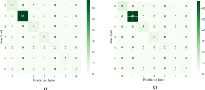
The confusion matrix for the proposed VotingR1 in (a) and VotingR2 in (b).
Scenario G: SHAP implementation and feature interpretability
This scenario introduces SHAP analysis to obtain feature-level interpretability for the best-performing ensemble model (VotingR2). Interpretability is essential for real-world decision-making, as policymakers require transparent explanations for why forecasts increase or decrease under certain conditions.
The SHAP summary plot (Fig. 12) illustrates both the magnitude and direction of feature effects. Cost is clearly the dominant predictor, exerting a strong positive influence on the predicted tourism numbers—consistent with the results observed in Sect. 4.1–4.5. Year ranks second, capturing long-term temporal trends, while City and Month contribute smaller but meaningful variations associated with local and seasonal patterns.
Overall, the SHAP analysis validates that the ensemble model’s predictions align with known economic and temporal dynamics in tourism. It also confirms that the model effectively captures both broad trends and localized fluctuations, strengthening confidence in its applicability for policy analysis and operational forecasting.

SHAP summary plot illustrating the relative importance and direction of feature contributions to the ensemble model’s predictions. Each dot represents an individual observation, where the horizontal axis denotes the SHAP value (impact on model output) and color intensity reflects the feature value (blue = low, red = high). Cost exhibited the highest positive contribution to tourism demand predictions, followed by Year, City, and Month, indicating that economic and temporal factors are dominant drivers in the model’s decision process.
Summary discussion
The results presented in Sect. 4.1–4.8 demonstrate that accurate tourism forecasting requires rigorous preprocessing, thoughtful model selection, and thorough evaluation across diverse forecasting conditions. While classical statistical approaches were effective in capturing broad temporal trends, machine-learning and ensemble methods, especially stacking and hybrid models, showed superior capability in modeling nonlinear relationships, seasonal effects, and complex interactions, resulting in the lowest forecasting errors. The observed seasonal fluctuations and distribution shifts also underscore the critical role of feature engineering and season-aware modeling in achieving robust and reliable predictions.
Beyond statistical accuracy, the results carry clear practical implications. Reliable forecasts can support infrastructure planning by helping authorities anticipate hotel, transport, and service capacity needs during peak and off-peak periods. They also enable targeted tourism marketing by identifying growth periods and regional demand trends, and contribute to economic diversification strategies by projecting tourism’s role in non-oil revenue expansion. Thus, the integrated hybrid modeling framework is not only technically effective but also well suited for real-world decision-making and long-term tourism policy development.