

To showcase the proposed design procedure, the Fisher’s 1936 iris flower classification is chosen as a dummy task, given its reputation as a well-known machine learning classification benchmark. This dataset contains 150 different flower specimens, each with 4 variables representing the dimensions of specific features, namely sepal length (SL), sepal width (SW), petal lengths (PL), and petal widths (PW) of multiple iris flower specimens. The dataset also includes three iris species classes, namely Setosa, Virginica, and Versicolor32. With these variables as inputs, we can create an architecture that can classify the 150 iris flowers into their respective 3 species.
To start, the values of the iris dataset should be modulated into a waveform by altering the amplitude of the four variables using four phasors with different frequencies, as shown in the Eq. (15).
$$\begin{aligned} v
(15)
The variables \(A_{SL}\), \(A_{SW}\), \(A_{PL}\), and \(A_{PW}\) represent the corresponding inputs, while \(f_1\), \(f_2\), \(f_3\), and \(f_4\) denote the phasor frequencies, which are 1 GHz, 1.2 GHz, 1.4 GHz, and 1.6 GHz, respectively. These frequencies collectively contribute to the signal periodicity with a period of 5 ns. It is important to note that these frequencies were selected based on our discretion, and they are not predetermined or forced. This is because although the data have to be modulated in a signal for this particular case, in electromagnetic classification problems, the data are automatically modulated in such signals. Samples of the modulated voltage waves from each class can be seen in Fig. 4a,b,c.

Iris Sample Signals and Circuit Response. This figure presents the iris sample signals for (a) Setosa, (b) Versicolor, and (c) Virginica. It also demonstrates the response of the circuit in Fig. 7 to the Setosa sample signal in (a) at the output nodes for (d) Setosa, (e) Versicolor, and (f) Virginica. Additionally, the figure illustrates the sampled voltage of the output nodes when they are stimulated with sample signals from (g) Setosa, (h) Versicolor, and (i) Virginica, which correspond to the signals shown in (a), (b), and (c), respectively.
It is essential to note that every neuron in the network must have the same specific input value. Without this, the neural network’s results will not be trustworthy. While it is easy to achieve this in software implementations, it requires careful attention in hardware implementations. Unwanted reflections can cause imbalances in the input signals received by each MIN. To ensure that the input is equally distributed and separated across all MINs, a power divider can be used. This component divides and allocates the input data into equal segments. To account for its scattering behavior, a new dataset should be derived from the original iris dataset. In the new dataset, each input value is divided by the \(\sqrt{3}\).
Using the backpropagation method, a layer consisting of 3 neurons was trained with the sigmoid as transfer function. Afterward, all weights are normalized according to the greatest weight which is \(-2.111022\) to include PIC by dividing all weights by its absolute value (2.111022). Table 1 displays the calculated and implemented weights, bias, and accuracy in each case. For implementation, weights with values such as \(|w_i|\simeq 1\) or \(w_i\simeq 0\) are rounded for simplicity of implementation. The accuracy values in Table 1 indicate that variations in weight values do not affect classification accuracy as long as the relationship between the output node values remains unchanged and the node with the highest value determines the class. Therefore, we can normalize the weights to the highest value node, which is useful when using special microwave devices like passive devices. This also suggests that small variations in implemented weights during manufacturing have negligible effects on the overall accuracy of the system.
It is important to note that the sigmoid function exhibits a strictly increasing behavior. Consequently, despite its utilization in the training phase, and given that the network in question is a shallow one-layer network, it can be disregarded during the implementation stage. Instead, the focus can be exclusively directed towards the values of the implemented nodes for the purpose of classification. In other words, the node possessing the highest positive value is attributed as the representative class without implementation of sigmoid function at hardware level.
The derived calculations suggest that a neuromorphic device tailored for iris dataset classification requires four ports, with one designated for input and the other three allocated for each class within the dataset. These port configurations correspond to the specific scattering parameter values outlined in Table 1. According to Eq. (9) the expected relevant scattering parameters of the device with ideal power combiners are represented by Eq. (16) through (18), and they are visually depicted with separate magnitude and phase plots in Fig. 5, where negative values are represented with \(180^\circ\) phase.
$$\begin{aligned} s_{21}= & \, 0.5\delta (f-1)-0.8\delta (f-1.4)-\delta (f-1.6) \end{aligned}$$
(16)
$$\begin{aligned} s_{31}= & \, 0.2\delta (f-1)-0.2\delta (f-1.2)+0.15\delta (f-1.4) \end{aligned}$$
(17)
$$\begin{aligned} s_{41}= & \, -0.7\delta (f-1.2)+0.5\delta (f-1.4)+\delta (f-1.6) \end{aligned}$$
(18)

Expected and simulated scattering parameters of a neuromorphic device for classifying iris dataset.
A microwave hardware can be designed in various ways to meet the expected scattering parameters in Eqs. (16) through (18). However, a simpler way to design it is to use three separate 2-port MINs instead of a single 4-port microwave device. To implement a 2-port MIN, directional couplers can be used since they affect the amplitude of phasors at each frequency, thereby eliminating the need for the phase correcting stage. A directional coupler is a 4-port microwave component in which the power applied to port 1, is transferred to port 3 (the coupled port) with a coupling factor of \(C^2\) (\(0<C<1\)), while the remaining input power is directed to port 2 (the through port) with a coefficient of \(D^2=1-C^2\). In an ideal directional coupler, no power is transmitted to port 4 (the isolated port)30.
The idea here is to use the coupling effect as a weight in a neuron, or \(w_i = C_i\) where \(w_i\) is a weight and \(C_i\) is the corresponding coupler’s coupling factor. For each weight, a specifically designed coupler can be utilized. If \(v_i
(19)
which at periods or \(t=T\) is equivalent to \(v_{o2}=A_1w_1+A_2w_2+\dots +A_nw_n+w_0\) that has the same form of Eq. (1). Therefore, by sampling \(v_{o1}\) at periods, a single neuron can be implemented using a network of directional couplers, microwave filters and phase shifters. This architecture, known as hybrid coupler network, is incredibly easy to design and fabricate, and the costs associated with manufacturing it are significantly low.
Figure 7 illustrates the suggested microwave design for the neural network based on hybrid coupler network. It uses suitable impedances for port matching, isolators to prevent undesirable reflections and separate MINs, band pass and band stop filters to gather data points at specific frequencies, and phase shifters to incorporate the negative weight values. Considering the utilization of power combiners at the termination of each branch to combine the individual voltage waves, it becomes imperative to account for their associated gain. This can be achieved by appropriately dividing the bias based on the scattering parameters of the power combiner. Referring to Fig. 7, it is essential to divide each bias by a factor of \(\sqrt{3}\). Thus, the biases in the normalized section of Table 1 are also divided by \(\sqrt{3}\). In addition, the biases also scaled to include DC voltage distribution between \(R_{eq}\) and \(R_L\) in implemented section of Table 1. The scattering parameters of the circuit in Fig. 7 are shown in Fig. 5 with blue lines in which the power combiners are considered ideal. In this case, nonideal power dividers or power combiners would result in a consistent decrease across all nodes and frequencies, ensuring a consistent relationship between the output values at each node.
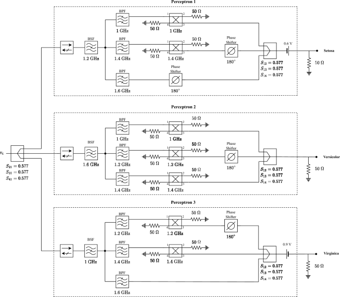
Microwave implementation of neural network with 3 neurons at the output layer.
When v(t) in Eq. (15) is given to the circuit shown in Fig. 7, the output signals at the Setosa, Versicolor and Virginica nodes take on the form of \(v_{o1}\) in Eq. (19). This output matches the output of the trained neurons when \(t=nT\). By sampling the output signals every 5 ns, the neural network’s output can be obtained, and ultimately solve the classification problem. The node with the highest sampled voltage determines the class.
Figure 4d,e,f show output signals at the Setosa, Versicolor, and Virginica nodes when the circuit is fed with the sample signal in Fig. 4a, which belongs to the Setosa class. At a time of \(t=5\) ns, the voltage at the Setosa, Versicolor, and Virginica nodes are 0.61, 0.18, and -0.82 volts, respectively. Based on this, the input signal is classified as Setosa, which has the highest voltage. Figure 4g,h,i show the output signals at the Setosa, Versicolor, and Virginica nodes when fed with signals in Fig. 4a through c, respectively, with the classified signal having the highest voltage value.
When comparing this work to similar works in33,34, it becomes clear that there are distinct differences in approaches and performances. The hybrid coupler network relies on passive components such as directional couplers, microwave filters, and phase shifters for computation. This leads to no power consumption for matrix multiplications since all the required power is derived from the input signal’s power. Passive devices typically demonstrate this type of performance. Nonetheless, when compared to similar devices like memristors, passive devices are significantly easier to design and manufacture. Moreover, the costs related to producing passive devices are much lower than those associated with memristors. While it is not reconfigurable or programmable, it can perform calculations of a shallow neural network independent from hardware. In other words, even though the footprint scales with input dimension, energy consumption, and calculation speed are not dependent on it. PCA also can be integrated into the hybrid coupler network; however, although the speed of calculation is not affected by the integration, the power consumption will scale according to the mean value of inputs. In addition, the data are transmitted through electromagnetic signals, eliminating the need for data modulation for electromagnetic classification problems resulting in an end-to-end system; however, for other problems, data modulation is necessary. The hybrid coupler network is cost-effective and easy to fabricate. It achieved an accuracy rate of 96.7% on the iris dataset.
In contrast33, uses ONNs (Optical Neural Networks) in the photonic domain, and uses light intensity modulated data. It is a one-layer network, with calculation speed limited by electrical equipment but it can be accelerated with high-speed programmable modulators and detectors. It uses ultracompact diffractive cells and slab waveguides to replace Mach–Zehnder interferometers (MZIs). The energy consumption and footprint scale linearly, and it operates with low power in the mW range. It also has an accuracy rate of 96.7% on the iris dataset.
34 utilizes vertical-cavity surface-emitting lasers (VCSELs) and photonic spiking neural networks (SNNs) with a larger number of nodes. It is highly hardware-friendly, inexpensive, and operates at low power (sub-mW). It provides full control over the number of interconnected spiking nodes and has a higher accuracy rate of over 97% on the iris dataset. Data modulation occurs through the intensity of light.
These comparisons highlight the differences in technological approaches and performance characteristics including factors such as reconfigurability, programmability, network depth, speed limitations, energy consumption, footprint scalability, cost, accuracy on the iris dataset, and data modulation methods.


