Appendix A Experiment details
Image classification
Datasets, data splits, preprocessing, and augmentation
Datasets: For the image classification experiments we use four datasets, two datasets with 32x32x3 pixel images and two datasets with 256x256x3 pixel images. For the 32x32x3 pixel images, the CIFAR-10 and CIFAR-10042 datasets were used. CIFAR-10 includes 60,000 images across 10 classes, while CIFAR-100 also contains 60,000 images of the same resolution, but categorized into 100 classes for a more detailed classification. For the 256x256x3 pixel images the Oxford Flowers43 and UC Merced44 datasets were used. Oxford Flowers comprises 8,189 images of varying dimensions across 102 classes, and UC Merced features 2,100 images divided into 21 classes.
Data Splits: In our experiments, the CIFAR-10 and CIFAR-100 datasets were divided into train, validation, and test sets containing 45,000, 5,000, and 10,000 images respectively, following the instructions by He et al.39. The Oxford Flowers dataset features a test set of 6,149 images and equal-sized training and validation sets of 1,020 images each. To improve accuracy, the test set was repurposed for training, and the training set for testing. For the UC Merced dataset, which does not have predefined splits, we applied a 70%/10%/20% split for training, validation, and testing.
Image allocation to each split in the CIFAR-10, CIFAR-100, and UC Merced datasets was achieved through a one-time random selection process. We ensured a uniform distribution of images across labels within these splits. Consistency was maintained by allocating the same images to the same splits in every training run.
Preprocessing: Image preprocessing involved normalizing the color channels based on the mean and standard deviation calculated across the entire dataset. For Oxford Flowers and UC Merced, images were further processed by resizing to 224x224x3, employing ”nearest” interpolation.
Augmentation: Data augmentation techniques were consistently applied across all training datasets in our experiments, following the methods outlined by Lee et al.56 and recommended by He et al., to improve model robustness and generalization.
Models
The ResNet models were developed using the PyTorch framework, following the protocols specified by He et al. The 20, 56, and 110 layer versions were used for the 32x32x3 pixel images, while the 18, 50, and 101 layer versions were used for 256x256x3 pixel images.
We used the ViT models from Hugging Face’s Timm libraryFootnote 1. We used the ViT-Small40 (ViT-S), and ViT-Base41 (ViT-B) variations with patch size 8 for the 32x32x3 pixel images. We used the ViT-Tiny40 (ViT-T), ViT-Small (ViT-S), and ViT-Base (ViT-B) with variations with patch size 16 for the 256x256x3 pixel images. Diverging from the approach in the original paper by Dosovitskiy et al., these experiments performed model training with random weight initialization rather than using pre-trained weights from the ImageNet and JFT datasets. This difference led to top-1 accuracy metrics that are notably lower compared to those achieved by the ResNet models and those reported by Dosovitskiy et al., who used pre-trained weights. Dosovitskiy et al. noted the challenges Vision Transformers face in generalizing effectively with limited data, recommending training on substantially larger datasets (ranging from 14M to 300M images) to achieve optimal performance.
ViT models were also trained using pretrained weights from the Timm library. These pretrained weights were not used with the 32x32x3 pixel images due to the requirement of image dimensions of 224x224x3.
See table 8 for the number of parameters in each model.
Hyperparameters
For experiments involving ResNet models with the CIFAR-10 and CIFAR-100 datasets, we adhered to the hyperparameters specified by He et al. in section 4.2 of their publication.
For other model and dataset configurations, hyperparameters were optimized through a systematic grid search, covering variations in learning rate, batch size, and optimizer choice. Learning rates tested were 0.1, 0.01, 0.001, and 0.0001; batch sizes considered were 32, 64, 128, and 256; and the optimizers evaluated included Stochastic Gradient Descent (SGD) and Adam.
Additionally, all models incorporated learning rate decay, with a decay factor of 0.1 applied after 50% and 75% of the total epochs were completed. The ResNet 110 models implemented a five-epoch learning rate warm-up at 0.1, following He et al.’s recommendation, due to the model’s initial difficulty in converging.
Models were trained for 200 epochs using random weights and 50 epochs with pretrained weights.
See table 9 for the hyperparameters used.
Time series forecasting
Datasets
In our time series experiments, we utilized six datasets:
The four ETT (Electricity Transformer Temperature) datasets49 are aimed at evaluating forecasting models for monitoring transformer temperatures. ETTh1 and ETTh2 feature hourly data with 7 variates across 17,420 timesteps. ETTm1 and ETTm2 provide data every 5 minutes, also with 7 variates, across 69,680 timesteps.
The Traffic dataset, sourced from the California Department of Transportation, records sensor data on freeways in the San Francisco Bay area, with hourly granularity, 862 variates, and 17,544 timesteps. The Weather dataset comprises various indicators recorded in Germany in 2020, detailed every 10 minutes, with 21 variates and 52,696 timesteps. Both the Traffic and Weather datasets were preprocessed as described by Wu et al47.
Forecasting horizons of 96, 192, 336, and 720 time steps were used for iTransformer, NLinear, and TSMixer models, aligning with published results. To maintain consistency across all models, these same horizons were applied to the Autoformer, deviating from the original authors’ approach. A uniform sequence length of 96 was utilized for all four models, corresponding to the published parameters for Autoformer and iTransformer. This standardization ensures comparability of results across the different models.
Models and hyperparameters
All models utilized in our study were trained using code provided by the authors, available on GitHub:
Each GitHub repository contained scripts to run the experiments, including predefined hyperparameters as documented in their respective publications. Modifications were made to the original code to ensure deterministic training, setting random seeds, and saving the outcomes.
We considered CNN time series models, like SCINet57 and TiDE58, however we chose not to use them in our experiments due to the long training times.
See table 10 for the number of parameters in each model.
Training
All Image Classification and Time Series models were trained deterministically one hundred times using the same one hundred randomly selected seeds. Deterministic training was enforced through framework-specific mechanisms for PyTorch and TensorFlow. For PyTorch, torch.use_deterministic_algorithms(True) was called prior to each run, forcing all applicable CUDA operations – including convolutions, scatter operations, and matrix multiplications – to use deterministic algorithms and raising a RuntimeError if no deterministic implementation is availableFootnote 2. The CUBLAS_WORKSPACE_CONFIG=:4096:8 environment variable was also set to ensure deterministic cuBLAS behavior, as required for CUDA versions 10.2 and above. cuDNN autotuning was not enabled (torch.backends.cudnn.benchmark defaults to False in PyTorch 2.2), preventing hardware-dependent algorithm selection across runs. For TensorFlow, tf.config.experimental.enable_op_determinism() was called to enforce deterministic op executionFootnote 3, and PROTOCOL_BUFFERS_PYTHON_IMPLEMENTATION=python was set to ensure consistent protobuf serialization behavior across nodes. In both frameworks, the random states of Python, NumPy, and the respective framework were seeded identically at the start of every run. Together, these settings ensure that observed variation across the 100 seed replicates reflects seed-based non-determinism only, and not uncontrolled implementation-level sources of variation.
When using the HPC system for training, deterministic results across each node were verified by training the models for one epoch using the same random seed and validating the top-1 accuracy results were the same.
Software environment
All the experiments were conducted within a software environment derived from Nvidia NGC containers available from https://docs.nvidia.com/deeplearning/frameworks/. To accommodate the HPC user security requirements, the Docker containers were converted to Apptainer containers. Version 23.12 of the TensorFlow and PyTorch containers was utilized. The TensorFlow container includes TensorFlow version 2.14.0, while the PyTorch container includes PyTorch version 2.2.0. Both containers are built on an Ubuntu 22.04 base and incorporate Python 3.10, CUDA 12.3.2, and cuDNN 8.9.7.29.
Appendix B Regularization method search
Regularization is a method identified by Dietterich36 to increase robustness of machine learning models. There exists little published research on regularization methods developed specifically for time series forecasting methods. We reviewed four survey papers51–54 on regularization methods for deep learning and selected ten regularization methods that were listed in two or more of the survey papers. We then did a Scopus search for publications with ”deep learning” OR ”neural network” and the ten regularization methods: ”L1 regularization”51–54 OR ”L2 regularization” OR ”weight decay”51–54 OR ”dropout”51–54 OR ”early stopping”51–54 OR ”batch normalization”51–54 OR ”data augmentation”51–54 OR ”adversarial training”51,54 OR ”label smoothing”51,54 OR ”multi-task learning” OR ”multitask learning”51,54 OR ”noise injection”51,54 returned 12704 papers with ”image AND (classification OR segmentation)” in the title, abstract, or keywords, while only 710 papers had ”time-series AND (forecasting OR prediction),” see Fig. 7.
Appendix C Additional Tables
Image classification
Time series forecasting
Appendix D Additional Figures
Image classification (Figs. 8, 9, 10, 11, 12, 13)

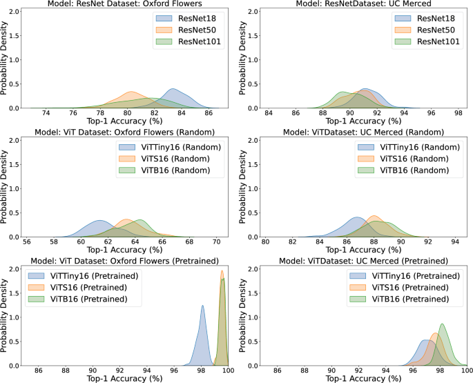
Kernel density estimates of top-1 accuracy for image classification models on Oxford Flowers (left) and UC Merced (right). Top row shows ResNet architectures (ResNet18, ResNet50, ResNet101); middle row shows Vision Transformers with random initialization (ViT-Tiny-16, ViT-S-16, ViT-B-16); bottom row shows Vision Transformers with pretrained weights (ViT-Tiny-16, ViT-S-16, ViT-B-16). Each curve represents the distribution across 100 random seeds for a single model-dataset pair.
Time series forecasting

Kernel density estimates of MAE for time series forecasting models on ETTh2 across forecast horizons of 96, 192, 336, and 720. Each panel shows distributions for Autoformer, iTransformer, NLinear, and TSMixer. Each curve represents the distribution across 100 random seeds for a single model-horizon pair.

Kernel density estimates of MAE for time series forecasting models on ETTm1 across forecast horizons of 96, 192, 336, and 720. Each panel shows distributions for Autoformer, iTransformer, NLinear, and TSMixer. Each curve represents the distribution across 100 random seeds for a single model-horizon pair.

Kernel density estimates of MAE for time series forecasting models on ETTm2 across forecast horizons of 96, 192, 336, and 720. Each panel shows distributions for Autoformer, iTransformer, NLinear, and TSMixer. Each curve represents the distribution across 100 random seeds for a single model-horizon pair.

Kernel density estimates of MAE for time series forecasting models on Traffic across forecast horizons of 96, 192, 336, and 720. Each panel shows distributions for Autoformer, iTransformer, NLinear, and TSMixer. Each curve represents the distribution across 100 random seeds for a single model-horizon pair.

Kernel density estimates of MAE for time series forecasting models on Weather across forecast horizons of 96, 192, 336, and 720. Each panel shows distributions for Autoformer, iTransformer, NLinear, and TSMixer. Each curve represents the distribution across 100 random seeds for a single model-horizon pair.
Appendix E Gradient dynamics and loss surface curvature (Figs. 14, 15)

Mean gradient L2 norm (left) and within-epoch gradient norm variance (right) across 200 training epochs for ResNet110 and ViT-B-8 on CIFAR-10, computed over 100 seeds. Shaded bands indicate the interquartile range across seeds. Dashed vertical lines mark learning rate decay events at epochs 100 and 150.

Perturbation-based sharpness at convergence for ResNet110 and ViT-B-8 on CIFAR-10, computed over 100 seeds. Each box shows the median, interquartile range, and 1.5 x IQR whiskers; points beyond the whiskers are plotted individually.
We conducted an exploratory analysis of gradient norm variance and loss surface curvature for ResNet110 and ViT-B-8 on CIFAR-10, computed over 100 seeds. For each seed replicate, we logged the mean and within-epoch variance of the gradient L2 norm at every epoch, and computed a perturbation-based sharpness measure at the end of training following59. Sharpness was defined as the relative increase in validation loss under a random weight perturbation of norm \(\epsilon = 10^{-4}\), averaged over ten perturbation samples per seed.
Figure 14 shows the gradient dynamics across 200 training epochs. ViT-B-8 exhibits a mean gradient norm approximately 3\(\times\) higher than ResNet110 during the first 25 epochs, after which both models converge to comparable values near 0.5. Within-epoch gradient norm variance collapses rapidly during the first ten epochs for both architectures; ResNet110 begins with a much larger initial spike than ViT-B-8. The IQR bands across seeds are tight throughout, indicating that these dynamics are consistent across random initializations.
Figure 15 shows the final sharpness values across 100 seeds for each model. Both models are centered near zero sharpness (scale \(\times 10^{-5}\)), with no large difference in central tendency, although ResNet110 appears to show somewhat greater variability across seeds.
These results suggest that gradient norm variance and loss surface curvature do not, by themselves, explain the differences in performance distribution spread between these architectures reported in Table 11. The robustness differences observed between ResNet110 and ViT-B-8 are not clearly matched by differences in late-training optimization dynamics, indicating that the distributional differences may instead reflect architecture-specific sensitivity to initialization or early training trajectory.

