Design/Setting/Participants
This retrospective study used the Nationally Designated Intractable Disease Database established based on Japan’s Intractable Disease Medical Care Act.20. The Japanese physician registration system and subsidy system for designated intractable diseases are as described above.20. This research was provided by the Ministry of Health, Labor and Welfare based on an application from the Ministry of Health, Labor and Welfare, using anonymized data based on designated intractable disease diagnosis certificates of newly registered patients from FY2015 to FY2021. Patients diagnosed with ADPKD and meeting the criteria for an intractable disease9 Apply for medical expenses subsidy from the government and be registered in the incurable disease database15, 20. The criteria for designating ADPKD as an intractable disease in Japan are as follows. (1) Red area of CKD severity classification in Kidney Disease Improvement Global Outcomes (KDIGO) heat map (patients with advanced stage CKD or severe proteinuria)twenty one (2) Total kidney volume (TKV) is 750 mL or more and TKV increase is 5% or more per year.9. This study was conducted in accordance with the 1964 Helsinki Declaration and its later amendments or comparable ethical standards. This study was approved by the institutional ethics committees of the Japanese Society of Nephrology (approval number: 70) and Juntendo University (approval number: 2021016), and the requirement for individual consent for this retrospective analysis was waived due to the characteristics of the data.
The study enrolled 2,737 patients who completed their initial application during the study period, and their CKD stage G classification (classified by GFR) was assessed at renewal application three years later. The database consists of baseline data collected during initial case enrollment and annual follow-up data recorded thereafter. Since each follow-up entry contained only one measurement taken by the attending physician, no preprocessing was applied and the recorded values were directly used as features. Using this data source, we constructed a dataset in which the clinical characteristics recorded at the time of the initial application were specified as predictors and the CKD stage determined at the 3-year renewal application was defined as the outcome.
Results evaluation
The primary endpoint was CKD stage G classification assessed after 3 years. Both CKD stage G and A classifications serve as severity criteria for determining whether a patient is eligible for financial support for incurable diseases in Japan, and are important indicators that influence clinical management. Among these indicators, the G classification is widely incorporated into mandatory health examinations and frequently measured in daily clinical practice, making it advantageous as ground truth data for machine learning analysis.
statistical analysis
Descriptive statistics were calculated for all predictor variables to assess the distribution of the data. Discrete variables were summarized by frequencies and percentages, and continuous variables were characterized by means and variances. Additionally, the number of observations for each variable was recorded. All analyzes were performed using R version 4.4.2.
Model fitting and evaluation
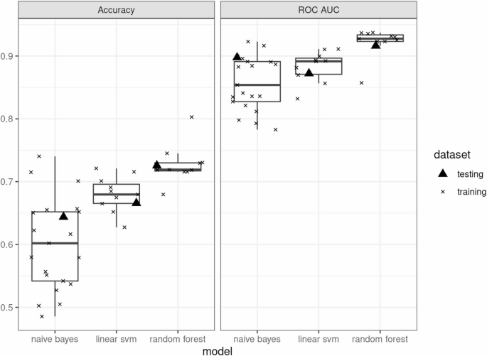
A classification model was developed to predict CKD stage 3 years after first application using clinical characteristics at the time of first application as input variables. Machine learning techniques considered included Naive Bayes models, linear support vector machines, and random forests. Stratified sampling was performed according to the 3-year outcome of CKD stage G classification, and then patients were assigned to a training set for parameter optimization (60%) and a test set for external validation (40%). The training set was utilized to generate multiple samples through k-fold cross-validation, allowing for the identification of parameters that exhibit stable performance across diverse datasets. The accuracy and ROC-AUC of the final model were calculated using a test set that was not involved in parameter optimization to evaluate its predictive performance. ROC-AUC represents the area under the receiver operating characteristic curve and serves as an indicator of the model’s ability to assign a high probability to the correct label.
Hyperparameter tuning of the training set was performed using a grid search with five candidate values defined for each parameter. For a random forest model, the grid includes the number of explanatory variables used in each tree (mtry: {4, 19, 35, 50, 66}), the number of trees (trees: {1, 500, 1000, 1500, 2000}), and the minimum number of observations required for a terminal node (min_n: {2, 11, 21, 30, 40}). Contains. This results in 125 hyperparameter combinations (5 candidate values for each 3 parameters). For linear support vector machines, the grid has a cost parameter that controls the penalty for misclassification (cost: {0.000977, 0.0131, 0.177, 2.38, 32.0}) and a margin parameter that defines the distance to the separating hyperplane (margin: {0.00, 0.05, 0.10, 0.15, 0.20}) It consists of For the naive Bayes model, the grid included the smoothness parameter for probability density estimation (smoothness: {0.50, 0.75, 1.00, 1.25, 1.50}), the Laplace smoothing coefficient (Laplace: {0.00, 0.75, 1.50, 2.25, 3.00}), and the threshold for the correlation coefficient used in feature selection. (Thresholds: {0.00, 0.25, 0.50, 0.75, 1.00}).
When building models using the three machine learning techniques, preprocessing was tailored to the specific characteristics of each approach. Although Naive Bayes models can handle datasets with missing values, it is known that high correlations between predictor variables can negatively impact prediction performance. Therefore, if variables showed high correlation coefficients, one of the correlated variables was excluded during preprocessing. In contrast, support vector machine and random forest techniques cannot handle missing values, so continuous variables were imputed using the mean and discrete variables were imputed using the mode during preprocessing. Furthermore, it is known that the predictive performance of Naive Bayes models decreases when there is correlation between predictor variables. Therefore, one of the correlated variables was removed from the model if a high correlation coefficient was observed.
To observe the built model and evaluate the contribution of each feature to its prediction, the importance of permutation features was calculated. This method quantifies the importance of a feature by measuring the increase in prediction error after randomly shuffling the values of a particular feature.


