Machine learning model provides stress biomarkers for the classification of abiotic stress in Micro-Tom

Plant material

The experiment was conducted in a brickwork room at the São Paulo State University (UNESP), School of Agricultural and Veterinary Sciences, Jaboticabal, Brazil. Micro-tomato (Solanum lycopersicum L. cv. Micro-Tom) seeds were germinated in trays containing a substrate composed of a 1:1 mixture of Basaplant^® and vermiculite, with dolomitic limestone added at 5% by volume. Plants were cultivated under white fluorescent lighting with an irradiance of 80 µmol m ⁻² s ⁻¹, a 12-hour photoperiod, an average temperature of 21 °C, and an average relative humidity of 60%.

Fifteen days after sowing, seedlings were transplanted into Leonard pots containing vermiculite and a modified⁵⁷nutrient solution, as described by⁵⁸. The nutrient solution concentration was adjusted sequentially to 25% for 48 h, then 50% for another 48 h, before reaching a full concentration (100%), with weekly replacements maintaining a volume of 250 mL per pot per replacement.

Experimental design and treatments

A completely randomized 3 × 2 factorial design was employed, with the first factor corresponding to the stress agents (water deficit, salinity, and cadmium) and the second factor representing the stress intensities (moderate and severe), along with a control group.

Water deficit intensities were induced by adding polyethylene glycol 6000 to the nutrient solution, achieving osmotic potentials of 0.00 MPa (control), −0.40 MPa (moderate), and − 1.00 MPa (severe). Salinity stress intensities were established with nutrient solutions containing 0.00 mM NaCl (control), 40 mM NaCl (moderate), and 120 mM NaCl (severe). Cadmium stress was induced using nutrient solutions containing 0.0 mM CdCl₂ (control), 0.25 mM CdCl₂ (moderate), and 0.5 mM CdCl₂ (severe).

Sampling dates

Plants were exposed to stress conditions for a period of 10 days. At the end of the exposure period, leaf samples were collected from six plants per treatment and immediately frozen in liquid nitrogen. The samples were then stored in an ultra-freezer at −80 °C for subsequent analyses.

Lipid peroxidation

Lipid peroxidation was estimated based on thiobarbituric acid-reactive substances (TBARS)⁵⁹. Plant tissues were homogenized in a mortar with 20% (w/v) insoluble polyvinylpyrrolidone (PVPP) and 0.1% trichloroacetic acid (TCA). The homogenate was centrifuged at 10,000 g for 5 min. An aliquot of 250 µL of the supernatant was mixed with 1 mL of 0.5% TBA prepared in 20% TCA. The mixture was incubated in a water bath at 95 °C for 20 min, and the reaction was terminated by rapid cooling in an ice water-bath. The malondialdehyde (MDA) concentration was calculated using an extinction coefficient of 1.55 × 10⁵ mol⁻¹ cm⁻¹, with readings taken at wavelengths of 535 and 600 nm⁶⁰. Results were expressed as µmol g⁻¹ fresh weight.

Hydrogen peroxide content

The hydrogen peroxide (H₂O₂) content was determined following⁶¹. Initially, 0.250 g of plant tissue was ground in liquid nitrogen and homogenized in 0.1% trichloroacetic acid (TCA). The homogenates were centrifuged at 10,000 rpm for 15 min at 4 °C. The supernatant was then mixed with 100 mM potassium phosphate buffer (pH 7.5) and potassium iodide (KI) solution. Samples were incubated in darkness for 1 h on ice. Triplicate readings were performed at 390 nm, with results expressed as µmol g⁻¹ fresh weight.

Proline content

Proline concentration was determined according to⁶², with modifications. A 0.250 g sample of plant tissue was ground in liquid nitrogen to a fine powder and homogenized in 3% (w/v) sulfosalicylic acid. The extract was then filtered, and aliquots of crude extract, acetic acid, and acid ninhydrin solution containing 2.5% ninhydrin were pipetted into test tubes and vortexed. Samples were incubated at 100 °C for 1 h, cooled on ice, and mixed with toluene. After 20 s of vigorous shaking, triplicate readings were taken at 520 nm, and results were expressed as µmol proline g⁻¹ fresh weight.

Enzyme extraction and protein determination

Fresh plant material was ground in liquid nitrogen with a porcelain mortar and pestle and homogenized in a 100 mM potassium phosphate buffer (pH 7.5) containing 1 mM ethylenediaminetetraacetic acid (EDTA), 3 mM dithiothreitol (DTT), and 4% polyvinylpolypyrrolidone (PVPP). The mixture was centrifuged at 10,000 rpm for 30 min at 4 °C. Supernatants were aliquoted and stored at −80 °C for subsequent enzymatic assays⁶³. Protein concentrations were determined using the⁶⁴, with bovine serum albumin as a standard. Samples were mixed with Bradford reagent, incubated for 2 min, and readings were taken at 595 nm in triplicate, with results expressed as mg mL⁻¹.

Enzyme assays

Superoxide dismutase (SOD, E.C.1.15.1.1)

Superoxide dismutase (SOD) activity was determined spectrophotometrically using the nitro blue tetrazolium chloride (NBT) method⁶⁵. The assay mixture contained 50 mM potassium phosphate buffer (pH 7.8), 50 mM methionine, 10 mM EDTA, 1 mM NBT, 0.1 mM riboflavin, and the plant extract. One unit of SOD activity was defined as the amount of enzyme required to inhibit NBT photoreduction by 50% at 560 nm. Triplicate readings were taken, and SOD activity was expressed as U SOD mg⁻¹ protein min⁻¹.

Catalase (CAT, E.C. 1.11.1.6)

Catalase (CAT) activity was determined by monitoring H₂O₂ decomposition spectrophotometrically over 1 min at 240 nm in triplicate⁶⁶, with modifications by⁶³. The reaction mixture included 100 mM potassium phosphate buffer (pH 7.5) and 25 µL H₂O₂ (30% solution). Values were expressed as µmol H₂O₂ min⁻¹ mg⁻¹ protein.

Glutathione peroxidase (GSH-Px, E.C. 1.11.1.9)

Glutathione peroxidase (GSH-Px) activity was measured according to⁶⁷ with modifications. The reaction mixture contained the plant extract, 100 mM potassium phosphate buffer (pH 7.0), 3 mM EDTA, 0.24 U GR/mL, 10 mM reduced glutathione (GSH), and 1 mM sodium azide. Samples were incubated at 37 °C for 10 min, followed by the addition of 1.5 mM NADPH and 100 µL H₂O₂. NADPH oxidation was monitored over 5 min at 340 nm. GSH-Px activity was calculated using a molar extinction coefficient of 6.22 mM⁻¹ cm⁻¹⁶⁸. Triplicate readings were taken, with results expressed as µmol of NADPH min⁻¹ mg⁻¹ protein.

Ascorbate peroxidase (APX, E.C.1.11.1.11)

Ascorbate peroxidase (APX) activity was determined using a reaction mixture containing 80 mM potassium phosphate buffer (pH 7.0), 5 mM ascorbate, and 1 mM EDTA, maintained in a water bath at 30 °C⁶⁰. Following reagent pipetting, H₂O₂ and the plant extract were added to the cuvette. Absorbance changes were measured at 290 nm over 1 min in triplicate, and APX activity was expressed as nmol of ascorbate min⁻¹ mg⁻¹ protein.

Glutathione reductase (GR, E.C. 1.6.4.2)

Glutathione reductase (GR) activity was determined spectrophotometrically using a reaction mixture of 100 mM potassium phosphate buffer (pH 7.5), 1 mM 5,5’-dithiobis (2-nitrobenzoic acid) (DTNB), 1 mM oxidized glutathione (GSSG), 0.1 mM NADPH, and the plant extract. The rate of GSSG reduction was measured by monitoring the increase in absorbance at 412 nm over 1 min⁶³. GR activity was expressed as nmol of GSSG min⁻¹ mg⁻¹ protein.

Statistical analysis

Descriptive analysis and multiple linear regression

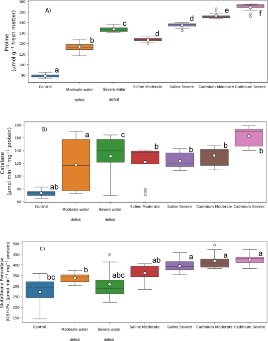
A Kruskall-Wallis factorial analysis of variance (ANOVA) was performed to assess the mean differences among the treatments for enzymatic, non-enzymatic systems, MDA and, H₂O₂, using a 5% confidence level (α = 0.05).

For each evaluation, 84 data points were collected across parameters including proline, CAT, GSH-Px, APX, GR, SOD, MDA, H₂O₂. Box plots were generated for each treatment (control, moderate water deficit, severe water deficit, moderate salinity, severe salinity, moderate cadmium, and severe cadmium) based on these parameters. Key statistical descriptors, including mean, median, maximum, minimum, quartiles, and variability, were represented in these plots. Additionally, the Shapiro–Wilk test was applied to assess the normality of stress indicators (MDA and H₂O₂).

To examine inter-variable relationships, an exploratory analysis was conducted using Spearman’s correlation on standardized data (expressed in standard deviations). Based on these correlations, a regression analysis was performed between MDA and H₂O₂ to understand treatment behavior for these stress indicators. Subsequently, multiple linear regression was applied to identify which factors (enzymatic and non-enzymatic systems) had the most significant influence on each stress indicator independently.

The Shapiro-Wilk test and the Spearman’s correlation were conducted using the pingouin (version 0.5.5) and the scipy.stats (version 1.14.1) libraries in the Python programming language.

All biochemical and stress-indicator datasets were inspected prior to modeling. No missing values were detected; therefore, no imputation procedures were required. For the machine learning workflow, biochemical variables (proline, CAT, SOD, APX, GSH-Px and GR) were standardized using z-score normalization.

Stress class creation

Quartile-based stress classes were established independently for each stress indicator (MDA and H₂O₂). For each indicator, quartiles (Q1, Q2, Q3) were calculated from the complete dataset, including all samples from water deficit, salinity, and cadmium treatments. Quartiles were selected as reference intervals because they are widely used for interpreting laboratory data⁶⁹. The following classes definitions were applied:

Machine learning model

The decision tree (DT) model was employed to classify stress levels in MT plants into four classes—low, low-average, high-average, and high—using the stress classes (target variable) derived from the levels of MDA and H₂O₂. The model used enzymatic and non-enzymatic antioxidant activity, as well as MDA and H₂O₂ data, as input features to build the classification model. The decision tree was chosen for its robustness, computational simplicity, and interpretative clarity⁷⁰, which allows not only for data classification but also for identifying key variables in the process.

The DT was constructed through homogenous data partitioning along predictor axes, creating subsets of the dependent variable (target) to classify new data⁷⁰. The architecture of the decision tree followed a top-down recursive partitioning approach, where at each node, the algorithm evaluated all possible splits of the predictor variables to select the split that maximized the homogeneity of the child nodes. The resulting structure consisted of a root node, multiple internal decision nodes, and terminal leaf nodes, each representing a final stress class assignment.

The DT classifier was implemented in scikit-learn (v1.1). All predictors were standardized before model fitting, and no missing values were present in the dataset. All 84 observations were used in training and validation through a fivefold cross-validation scheme. In each fold, 80% of the data were used for training and 20% for testing, ensuring that every sample contributed to both phases and enhancing the reliability of performance estimates for a small dataset. To prevent overfitting while maintaining model interpretability, the maximum tree depth was set to 4, as deeper configurations reduced cross-validated performance whereas shallower trees were unable to capture relevant nonlinear relationships among predictors. The minimum samples per split and per leaf were set to 2 and 1, respectively, allowing full exploration of the dataset given the depth constraint.

Model hyperparameters were tuned using GridSearchCV with fivefold cross-validation to ensure generalizability. The final model was trained using proline, CAT, GSH-Px, APX, GR, and SOD as input variables and the quartile-based stress classes for MDA and H₂O₂ as target outputs.

Machine learning model performance

A confusion matrix was generated to identify correct and incorrect classifications within the training dataset. The confusion matrix organizes data such that each column represents the model’s predictions, while each row represents a real sample label⁷¹. For the matrix evaluation, the following metrics were considered:

Where, TP is true positives, TN is true negatives, FP false positives, and FN is false negatives.

In this context:

• True positives (TP) are cases where the model correctly identifies a sample as belonging to a particular stress class.

• False positives (FP) are cases where the model incorrectly classifies a sample as belonging to a stress class when it does not.

• False negatives (FN) are cases where the model fails to classify a sample that truly belongs to a stress class.

• True negatives (TN) are cases where the model correctly identifies that a sample does not belong to a given stress class.

According to⁴⁷, precision (also known as positive predictive value) measures the proportion of true positives among all samples predicted as positive, highlighting the model’s ability to avoid false positives (overprediction). On the other hand, recall (also called sensitivity or true positive rate) measures the proportion of actual positives that the model correctly identifies, indicating the model’s ability to capture all relevant cases. These complementary metrics are often combined into the F1-score to provide a balanced evaluation of model performance.

The Matthews Correlation Coefficient (MCC) was used to evaluate overall model performance, with values ranging from − 1 to 1, corresponding to total misclassification and perfect classification, respectively⁴⁷. Additionally, the F1-score measures the model’s performance in classifying each class separately. For both tasks, training and evaluation, the scikit-learn library (version 1.1) was in Python programming language.