
The experimental test was carried out for 54 immature oocytes. At first, each oocyte was individually injected into the channel with a very low flow rate of about 0.05 µl per minute. The flow was then increased stepwise at intervals of 10 s. This time interval was to ensure whether the oocyte would pass through the channel at the applied flow rate or not. This process continued until ultimately, for a specific flow rate, the oocyte passed through the channel, and thus the critical flow for each oocyte was calculated.
Oocyte size is one of the parameters that can be analyzed as a characteristic in evaluating the oocyte. It should be noted that the size should be processed from the images of the oocyte before entering the trap channel (where the oocyte is almost spherical). For this purpose, the image was cropped so that only the desired cell remained in the frame. In the case of high-volume images, for example, when it is intended to process all the recorded images from the video, this is important because larger images require more processing time. Then, the center of the oocyte was identified in the binary image. In the next step, the number of pixels in the horizontal and vertical directions in the binary image was counted. After measuring the length (LO) and width of the oocyte (WO), the size of the oocyte is presented as the average of these two parameters as follows:
$$Size_{Oocyte} = \frac{{L_{o} + W_{o} }}{2}$$
(3)
The value of oocyte deformation is one of the parameters extracted in this study as a characteristic feature of the oocyte when subjected to critical flow conditions within the entrapment channel. A binary image of the oocyte at the threshold of entering the trap channel under critical flow (similar to the position considered for measuring surface stress) is used to measure this parameter. An image of the oocyte at the threshold of entering the channel under critical flow, along with its maximum length and maximum width, is depicted in Fig. 3g.
Therefore, based on the Fig. 3e, the deformability index (DI) is calculated as follows:
Furthermore, after proceeding with the biological experiments, the GV, MII, Zygote, and Cleaved Embryo stages were recorded as the fate of the development of oocytes in Supplementary Table S1. Also, the CT values for 54 oocytes at the GV stage are reported in Supplementary Table S1. Additionally, this table illustrates the critical pressure levels for various samples. It should also be noted that the oocyte’s passage speed remains nearly constant during its transit through the channel; thus, it can be assumed that the oocyte is trapped in a stable state during its passage through the channel (in terms of mechanical equilibrium—due to zero acceleration. Considering the above discussions, the features of size, CT, critical flow, and DI were measured for 54 immature oocytes at the GV stage.
Statistical analysis
This section focuses on the statistical analysis of the experimental data obtained from the study. As evident from Fig. 4a, the maturation rate in the experimental samples was 72%, indicating that a substantial majority of the collected immature GV oocytes were capable of progressing to the MII stage under the applied in vitro conditions. This maturation capability is a crucial indicator of oocyte developmental competence. Additionally, the fertilization rate was approximately 85%, suggesting that a high proportion of the matured oocytes retained functional integrity and were receptive to sperm penetration and subsequent zygote formation. Finally, 79% of the successfully fertilized oocytes reached the cleavage embryo stage, which signifies further embryonic development and is often considered a positive prognostic marker in assisted reproduction. Collectively, these developmental milestones reflect the biological relevance of the mechanical features studied in this work, validating their potential as predictors of oocyte quality and developmental fate.

(a) Maturation, Fertilization, and cleavage embryo stage. (b) The correlation between different features was analyzed using a Correlation Matrix and a Heatmap. (c–f) Distribution of key features including (c) Cell size, (d) CT, (e) Q, and (f) DI values. The histogram of cell size shows a concentration in the range of 105–115, indicating that most cells fall within this size range. The CT value distribution is primarily concentrated between 1 and 4, but with a wider spread for higher values. The Q value shows an asymmetrical distribution with a concentration around 0.1–0.5, suggesting low Q values for most cells. Finally, the DI distribution is focused between 1.2 and 1.3, implying relative consistency in this feature across the dataset.
Also, to analyze the data related to the evaluated cells, we employed both statistical and graphical methods to gain a deeper understanding of the key features. This analysis included examining the distribution of the data and investigating the correlation between variables. Initially, we assessed the distribution of four main features—Cell size, CT, Q, and DI values by utilizing histograms. These histograms provided us with valuable insights into the distribution patterns of each feature.
Figure 4b illustrates the histograms representing the distribution of four key features: Cell size, CT, Q, and DI. In general, a strong correlation between features indicates a direct relationship, meaning that an increase in one feature corresponds to a rise or decline in another. For instance, CT and Q have a very strong and direct correlation with a coefficient of 0.9, demonstrating a close relationship between the two. On the other hand, CT and DI show a significant negative correlation (-0.74), suggesting that an increase in CT leads to a decrease in DI. These correlation relationships highlight that some parameters have a greater influence on predicting cell categorization. For example, the strong correlation between CT and Q may play an essential role in predictive models, as a change in one is likely to lead to a similar shift in the other. Consequently, correlation analysis enhances the accuracy of predictive models and identifies which features are more relevant for future evaluations or machine learning models. In the next step, we analyzed the distribution of key features, including (Fig. 4c) Cell size, (Fig. 4d) CT, (Fig. 4e) Q, and (Fig. 4f) DI values. As shown in the figures, the Cell size feature exhibits a distribution concentrated within the 105 to 115 range, indicating that most cells fall within this size bracket. The CT values are primarily clustered between 1 and 4, though the distribution is skewed, with more scattered data points at higher values. Similarly, the Q feature exhibits a skewed distribution, with values concentrated between 0.1 and 0.5, suggesting that most cells have a low Q value. Lastly, the DI feature is concentrated between 1.2 and 1.3, indicating a relative uniformity in this feature across most cells. These distributions help us identify the overall behavior of the features and their potential impact on subsequent predictive models. The analysis of feature distribution and correlation provided valuable insights into the behavior and relationships among the various cell features. This information can aid in identifying hidden patterns within the data and contribute to better cell classification based on specific characteristics. Furthermore, the presence of correlations between features can serve as a guide for designing future experiments or refining predictive models.
Image processing
This section includes four steps, which are outlined below:
Local thresholding in images
In the first step, local thresholding method has been employed for oocyte identification. For example, consider the Fig. 5a as the initial input. Figure 5b shows the output image of this step. As can be seen from this figure, the edges of the oocyte and the channel walls are determined in this image.

Image processing steps. (a) A frame of oocyte on the verge of entering the trap channel. (b) Local thresholding stage in image processing. (c) Hole filling stage. The salt noise filter is applied at this stage. (d) Background image when no oocyte has entered the channel. (e) Stage of removing intersecting lines and background removal. In this image, the lines related to the channel have been removed. (f) Binary image of the detected oocyte after smoothing.
Filling holes
As depicted in Fig. 5b the oocyte in the previous stage was identified as hollow. In this step, to detect oocytes, the image was first binarized using the im2bw function with a threshold rate of 0.2, and then all the holes and closed curves were filled using the imfill (IMAGE2,‘holes’) function. In this stage, objects with an area smaller than 100 pixels were considered as noise and removed from the image (note that the area of the oocytes was greater than 300). For example, if the output of the image from the previous stage is used as the input of this stage, the result will be as shown in Fig. 5c. As is observed, the oocyte along with the remaining lines from the channel are clearly delineated. Moreover, all the noise has been removed from the image, leaving only the oocyte and the channel edges.
Removing intersecting lines and background image
As evident in the Fig. 5c, besides the oocyte, lines from the channel, mostly perpendicular or horizontal, connected to the oocyte remained. In this step, these lines were removed. Using the imclearborder (newImg, 18) function in MATLAB, any object connected to the edge of the image could be removed. In this stage, the background image was also removed by subtracting the images from the channel (when no oocyte had entered it). The background image and the output image are shown in Fig. 5d and e, respectively.
Smoothing the oocyte surface
As seen in Fig. 5f, the oocyte surface appeared uneven. To improve the clarity of the detected image and make it more similar to the oocyte image, the edges of the images were smoothed using the strel (‘disk’, 2, 8) function. Now this image is ready for extracting the required information.
Analysis and prediction of cell behavior using machine learning algorithms
In this study, both classification and clustering techniques were utilized to categorize and predict cell behavior based on various features. In the initial phase, we applied several classification algorithms, including Decision Tree, Random Forest, KNN, SVM, Naive Bayes, logistic Regression, XGBoost, and LightGBM, to the dataset. These methods were chosen for their strong performance in handling complex and nonlinear relationships within data. To evaluate the effectiveness of each classification method, we employed two validation techniques: LOO Cross-Validation and k-fold Cross-Validation. These methods allowed us to assess the accuracy and robustness of the models, helping us determine which algorithm produced the best predictive results for our dataset. The following sections provide a detailed analysis of the results obtained from both the classification and clustering methods, along with a discussion on their implications for cell categorization and prediction.
Phase I: classification algorithm
In the first phase, we focus on the implementation of various classification algorithms to analyze the mechanical properties of oocytes and their impact on cellular categorization. The objective is to leverage machine learning techniques to accurately classify oocytes based on their features, such as size, CT, and deformation under critical flow conditions. To achieve this, we employed several popular classification algorithms, including Random Forest, KNN, and XGBoost. These algorithms were chosen for their ability to handle complex datasets and their proven effectiveness in various classification tasks. The performance of each algorithm was evaluated through robust cross-validation methods, specifically K-fold and LOO validation, to ensure the reliability and generalizability of the results. The analysis begins with an examination of the correlation between key features, identifying significant relationships that may influence the classification outcomes. By training the algorithms on our dataset, we aimed to determine the most accurate model for predicting oocyte fate. This phase is crucial for establishing a foundation for subsequent analyses, where the insights gained will inform the understanding of oocyte behavior and enhance IVF outcomes. Overall, the implementation of classification algorithms in this phase highlights the potential of machine learning in improving the precision of oocyte assessments, ultimately contributing to advancements in reproductive technology.
Figure 6a illustrates a comparison of K-fold and LOO cross-validation results for classification algorithms. As shown in Fig. 6a (Left), in K-fold cross-validation, Random Forest achieves the highest accuracy at 75.96%, followed closely by KNN at 74.04%. Naive Bayes performs well with 70.19%, while SVM and Logistic Regression score 66.62% each. XGBoost achieves 68.41%, while Decision Tree lags at 64.56%. LightGBM has the lowest accuracy at 55.49%. This indicates that ensemble methods like Random Forest and KNN perform consistently well when trained on larger subsets of the data, whereas LightGBM struggles. Also, as shown in Fig. 6a (Right), in LOO cross-validation, KNN, Random Forest, and XGBoost all achieve the highest accuracy at 68.52%, showing a balanced performance. Naive Bayes follows closely at 66.67%, and Logistic Regression achieves 64.81%. SVM and Decision Tree perform similarly at 59.26%, and LightGBM shows a moderate improvement to 61.11%. The ensemble methods and Naive Bayes perform better in this setup, as they generalize well from the smaller data points used for training in LOO. Therefore, K-fold cross-validation favors Random Forest and KNN, which demonstrate strong performance when trained on larger portions of the dataset. In contrast, LOO validation highlights the strengths of ensemble methods like XGBoost and Random Forest, as these models adapt effectively to smaller training data points. LightGBM struggles in K-fold cross-validation but shows slight improvement in LOO, indicating its sensitivity to data partitioning. Given that Random Forest yielded the best results in our evaluation, we used this method to analyze the impact of different parameters. When comparing the Random Forest results using K-fold and LOO cross-validation, several insights emerged regarding the algorithm’s behavior and the importance of various features. The classification accuracy of the Random Forest algorithm based on different parameter combinations is presented in Fig. 6b. This figure demonstrates the accuracy rates achieved using both K-Fold and LOO validation methods. Notably, the combination of CT, Q value, and DI value achieves the highest accuracy of 76.10% in K-Fold validation, indicating the significant impact of these parameters on the model’s performance. We will now highlight these insights in the following:

(a) Comparison of K-fold and LOO Cross-Validation Results for Classification Algorithms. The chart illustrates the performance of various classification algorithms, including Random Forest, KNN, Decision Tree, SVM, Logistic Regression, Naive Bayes, XGBoost, and LightGBM. Results are displayed for two validation methods: (a) K-fold and (b) LOO. The accuracy varies across methods, with Random Forest and KNN performing best in K-fold, while ensemble models like XGBoost excel in LOO. LightGBM shows significant improvement in LOO compared to K-fold, where it performed the weakest. (b) Accuracy of Random Forest Classification Using K-Fold and LOO Validation. This chart illustrates the classification accuracy of the Random Forest algorithm based on various parameter combinations, evaluated using K-Fold and LOO methods. The combination of CT, Q, and DI yields the highest accuracy of 76.10% in K-Fold validation, showcasing the effectiveness of these features in enhancing classification performance.
Highest accuracy: In K-fold, the highest accuracy (76.10%) is achieved using the combination of “CT, Q, and DI.” In LOO, however, the highest accuracy (75.93%) is obtained with just “CT and DI.” This suggests that in K-fold, the “Q” feature adds value to the model’s performance, whereas in LOO, “Q” does not significantly enhance the model, and “CT and DI” alone are sufficient for optimal results.
Sensitivity to feature combinations: In K-fold, the inclusion of all parameters (Cell size, CT, Q, and DI) leads to an accuracy of 75.96%, slightly lower than using “CT, Q, and DI.” This suggests that in K-fold, adding “Cell size” can slightly dilute the performance. However, in LOO, using all four parameters leads to an accuracy of 68.52%, equal to several other combinations (e.g., “CT, Q, and DI” and “Cell size, CT, and DI”). This indicates that LOO is less sensitive to the number of parameters and more dependent on specific key features, such as “CT and DI.”
Performance drop with fewer features: In both K-fold and LOO, removing certain key parameters significantly impacts the model’s accuracy. For example, in K-fold, using only “CT and Q” results in an accuracy of 57.55%, while in LOO, the same combination drops even further to 48.15%. Similarly, “CT alone” yields weak results in both K-fold (57.55%) and LOO (46.30%). This suggests that “CT” is not a strong standalone feature in either validation method and requires the presence of “DI” for better performance.
Importance of the “DI” parameter: In both validation methods, the “DI” parameter plays a crucial role in improving accuracy. In K-fold, “DI” alone gives a relatively high accuracy of 66.48%, while in LOO, it also performs well with 66.67%. Additionally, “CT and DI” combinations show strong performance in both K-fold (68.54%) and LOO (75.93%). This consistency highlights “DI” as a critical feature across different cross-validation strategies.
Sensitivity of LOO to smaller feature sets: LOO tends to show more drastic fluctuations in accuracy when fewer parameters are used. For example, when only “Cell size and CT” are used, K-fold yields 62.77%, but LOO results in just 57.41%. This indicates that LOO is more sensitive to the loss of key features, particularly when the dataset is partitioned into very small training sets (as happens in LOO).
Therefore, “CT and DI” are crucial in both methods, but K-fold benefits more from additional features like “Q,” whereas LOO relies more on a few strong features. LOO is more sensitive to feature combinations and individual feature performance, as it works with fewer training data points at a time. K-fold generally shows more stable performance across different feature combinations, while LOO exhibits greater variability, with a steeper decline in accuracy when weaker features are used. In conclusion, while both methods highlight the importance of feature selection, LOO demonstrates a greater sensitivity to key features like “DI” and shows less improvement with the inclusion of secondary features like “Cell size” and “Q” compared to K-fold. The bar charts in Fig. 5b (both K-Fold and LOO CV) demonstrate how different combinations of CT and Q affect classification accuracy. For instance, the combination of CT, Q, and DI yields the highest K-Fold accuracy (76.1%), indicating that Q contributes complementary information despite its correlation with CT. Conversely, using CT or Q alone leads to slightly lower accuracy. These results suggest that while CT and Q are strongly correlated, their joint inclusion, particularly when combined with features like DI, enhances the model’s performance.
Phase II: clustering algorithm implementation
In the second phase of the analysis, we focused on clustering techniques to group similar data points. The clustering algorithms used were K-Means, DBSCAN, Agglomerative Clustering, and Gaussian Mixture Models. Each of these algorithms offered a unique perspective on the structure of the data and helped in identifying natural groupings among the samples. This comprehensive approach enabled us to understand the patterns and relationships within the data more effectively, guiding us toward more accurate predictive models for future work.
Supplementary Fig. S1 presents the results of clustering analysis using four different algorithms: K-Means, DBSCAN, Agglomerative Clustering, and Gaussian Mixture. The data points represent cell size and CT, which are the key features used in this analysis. Blue points indicate correctly clustered data, while gray points represent misclassified instances. K-Means, a widely used algorithm for clustering, shows some success in assigning correct clusters but also has several misclassifications. DBSCAN performed poorly in this study, struggling to correctly cluster the data and leading to a higher rate of misclassifications compared to other methods. Agglomerative Clustering, a hierarchical method, performs relatively better than K-Means and DBSCAN, with fewer misclassifications and a more accurate identification of clusters. The Gaussian Mixture algorithm, based on probabilistic models, also demonstrates good clustering accuracy but still exhibits some degree of error. Overall, this visual comparison of clustering performance aids in determining which algorithm best categorizes the oocyte data.
In evaluating the clustering performance of different algorithms, we utilized four key metrics: Silhouette Score, Davies–Bouldin Score, Calinski–Harabasz Score, and Adjusted Rand Index (ARI). Silhouette Score ranges from − 1 to 1, where values closer to 1 indicate well-clustered data, 0 indicates overlapping clusters, and negative values suggest incorrect clustering. Davies–Bouldin Score is non-negative and lower values indicate better clustering, with 0 representing perfectly separated clusters. Calinski–Harabasz Score has no fixed upper bound, and higher values indicate better-defined and more separated clusters. Adjusted Rand Index (ARI) ranges from -1 to 1, with 1 representing perfect agreement with ground truth, 0 indicating random labeling, and negative values suggesting worse-than-random clustering.
These metrics provide comprehensive insights into the quality of the clusters formed by each algorithm. Table 1 presents the performance comparison of the four clustering algorithms—K-Means, DBSCAN, Agglomerative Clustering, and Gaussian Mixture Models—across various evaluation metrics, including Silhouette Score, Davies–Bouldin Score, Calinski–Harabasz Score, and Adjusted Rand Index (ARI). This table provides a detailed overview of each algorithm’s ability to form well-defined clusters.
Among the algorithms, Agglomerative Clustering consistently outperformed others across multiple metrics. It achieved the highest Silhouette Score of 0.49, indicating well-separated clusters, and the lowest Davies–Bouldin Score of 0.73, signifying compact and distinct groupings. Its performance on the Calinski–Harabasz Score was also strong, with a value of 41.18, reflecting a good balance between cluster cohesion and separation. K-Means also demonstrated competitive performance, particularly excelling in the Calinski–Harabasz Score, where it achieved the highest value of 42.88. Additionally, K-Means performed well in the Silhouette Score (0.46) and Davies–Bouldin Score (0.88), showcasing its ability to form relatively distinct and well-separated clusters. However, it lagged slightly behind Agglomerative Clustering in these two metrics. The Adjusted Rand Index (ARI) further highlighted K-Means as the best performer with a score of 0.18, suggesting reasonable alignment between the predicted clusters and the true labels. Gaussian Mixture Models showed results comparable to K-Means in most metrics, achieving a Silhouette Score of 0.46, a Davies–Bouldin Score of 0.90, and a Calinski–Harabasz Score of 41.97. While its performance was solid, it did not significantly outperform either K-Means or Agglomerative Clustering. In contrast, DBSCAN struggled across all metrics. It produced a negative Silhouette Score (− 0.13) and a high Davies–Bouldin Score (1.8), indicating poorly defined clusters. Additionally, DBSCAN’s performance in the Calinski–Harabasz Score (1.54) and ARI (− 0.01) was notably low, suggesting that it failed to identify meaningful patterns in the dataset.
Overall, the analysis highlights Agglomerative Clustering and K-Means as the most effective methods for this dataset, with Agglomerative Clustering slightly edging out in cluster separation, while K-Means shows stronger performance in forming compact clusters and aligning with true labels. DBSCAN, on the other hand, is not well-suited for this clustering task, given its poor performance across all evaluation metrics. These results provide important insights for selecting appropriate clustering techniques in future analyses and predictive modeling efforts.
Although the focus of this study is biomechanical classification, preliminary tracking suggests that oocytes flagged as high-quality by the model tend to achieve higher fertilization and cleavage rates. A comprehensive statistical analysis linking these predictions to downstream embryonic and implantation outcomes is currently being planned and will be addressed in future work.
Assessment of method’s non-destructiveness via oocyte ultrastructure
The images related to this section are shown in Fig. 7A–F. This examination indicated that the cytoplasm of the oocytes remained intact, with uniformity preserved, and no signs of vacuolization were observed. The mitochondria were in a healthy state, with consistent sizes next to each other and interacting with other organelles. Cristae were uniform and regular, displaying the appearance of a healthy mitochondrion. The rough endoplasmic reticulum was well-visible in the cytoplasm, maintaining its connection with other intracytoplasmic components. Cortical granules (CG) were significantly produced in mature oocytes, accumulated beneath the oolemma. The oolemma remained relatively intact, and its microvilli were well-defined in the sub-zonal space. The sub-zonal space around the oocyte was uniform, with only minimal expansion observed in very limited areas. The zona pellucida section indicated its complete health, with its uniformity remaining untouched.
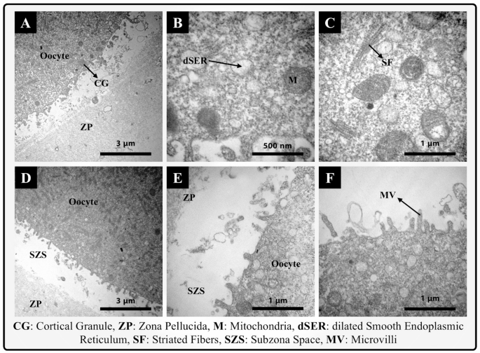
The assessment of the ultrastructure of an experimental oocyte after passing through the fabricated microfluidic chip.
Comparison of methods
While the integration of AI with dynamic imaging methods has recently achieved successes in selecting high-quality oocytes or embryos, all these evaluation models, whether static or dynamic, rely on large-scale morphological features of oocytes and embryos such as pronuclear position, cell number, fragmentation degree, blastocoel expansion rate, and the timing of specific events (cleavage, compaction, blastocoel formation initiation). This reliance leads to the complete disregard of other intracellular characteristics that are not visible with a conventional microscope. Also, dynamic imaging methods based on time-lapse microscopes are very time-consuming and expensive. To evaluate each oocyte, a full-time time-lapse imaging system needs to be dedicated solely to evaluating one oocyte. Moreover, these methods usually focus on evaluating embryos and have not been able to establish a relationship between oocyte quality and success in the IVF process. While evaluating oocytes in the early stages can significantly reduce ancillary costs such as maintenance, fertilization, and cultivation.
It has been proven that measuring the deformation of oocytes can provide insights into fundamental cellular processes such as migration, division, and signaling. The mechanical properties of cells are evaluated by measuring and analyzing the deformation of cells (oocyte resistance to deformation) when subjected to mechanical forces. In fact, evaluating the mechanical properties of cells requires describing the deformation of cells in response to mechanical forces over time, which can be described by the theory of stress and strain. Various parameters (such as Young’s modulus and CT) can be measured to calculate the mechanical properties of cells. To provide a more objective comparison, Table 2 summarizes key characteristics of three approaches used in oocyte and embryo assessment: static image-based AI methods, time-lapse microscopy (TLM)-based dynamic analysis, and our proposed microfluidic-AI integrated method. Unlike static microscopy, which relies solely on 2D morphological features such as solidity or circularity, and TLM which tracks developmental timepoints (e.g., time to polar body appearance), our method extracts mechanical features such as CT and DI during microfluidic passage. In terms of predictive performance, static AI methods such as those in Fjeldstad et al.21 report AUC values around 0.67, while TLM-based systems (Kalyani et al.36) have achieved classification accuracy up to 93% (sensitivity = 97%, specificity = 77%). Our method yields 76.1% accuracy (K-Fold CV) and 75.9% accuracy (LOO CV), with a minimal training dataset of just 54 oocytes. Importantly, while TLM systems require high-cost equipment (~ 100,000 USD), our method achieves real-time mechanical assessment using a low-cost microfluidic setup (~ 5,000 USD), comparable to static image systems. Additionally, it offers rapid analysis (~ 2 min per oocyte) without requiring long-term culture or multi-frame labeling.
These results support the practical superiority of our method in terms of cost-efficiency, speed, and reduced data requirements, while maintaining competitive classification accuracy compared to existing advanced techniques.”
In recent years, various methods have been used to evaluate the mechanical properties of oocytes, including the TMAM, atomic force microscopy, and microelectromechanical systems. In this study, a microfluidic channel was used to evaluate the mechanical properties of oocytes. Microfluidics, due to features such as rapid sample processing and precise flow control, can potentially serve as an alternative to conventional experimental methods.
In TMAM, measuring pressure is a difficult and complex process. We propose a simpler and more accurate process for measuring oocyte hardness using a microfluidic device. The oocyte trapping method in the proposed microfluidic device, using a hydrodynamic mechanism, is faster and more accurate compared to traditional methods, and significantly reduces human intervention.
Supplementary Fig. S2a illustrates the TMAM. The operation mechanism of this method is that initially, under the influence of a suction pressure, the cell is partially pulled into the micro-pipette. By applying pressure, the fluid level is displaced. By measuring this displacement, the fluid pressure is ultimately calculated through the equation P = ρgh. Any vibration or evaporation from the fluid surface can cause measurement errors. Additionally, this method requires high-quality equipment and technical skills. To the contrary, Supplementary Fig. S2b shows our proposed method. Based on the provided explanations, the pressure measurement process in this method is simpler. Unlike the TMAM, it does not require complex equipment. Additionally, there are no errors related to liquid surface evaporation and vibration, resulting in higher measurement accuracy. The measurement time in this method is less than five minutes, which is shorter compared to TMAM. Furthermore, the applied stress in this method is less than that in TMAM.


