With the idea of k-NN regressors and distance-based predictions in mind, let’s now look at k-NN classifiers.
Although the principle is the same, classification allows us to introduce several useful variations, such as radius nearest neighbor, nearest centroid, multiclass prediction, and stochastic distance models.
Therefore, we will first implement a k-NN classifier and then explain how it can be improved.
Use this Excel/Google Sheet while reading this article to better understand all the instructions.

Titanic survival dataset
We will use the Titanic survival dataset. This is a typical example where each row describes a passenger with characteristics such as class, gender, age, fare, etc., and the objective is to predict whether the passenger survived or not.

Principle of k-NN for classification
The k-NN classifier is so similar to the k-NN regressor that I could write an entire article to explain both.
When you actually search, k nearest neighbor, value not used y absolutely, Much less Its nature.
However, there are still some interesting facts about how classifiers (binary or multiclass) are constructed and how features are processed differently.
We start with a binary classification task and then do multiclass classification.
One continuous feature for binary classification
Therefore, you can quickly perform the same exercise on a single continuous feature using this dataset.
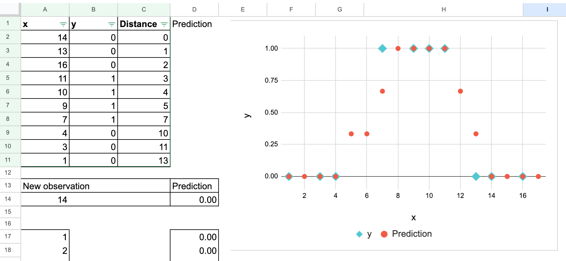
The values of y are typically 0 and 1 to distinguish between the two classes. But you can be aware that it can cause confusion.

Now, think about it. 0 and 1 are also numbers, right? So you can do exactly the same process as you are doing regression.
That’s correct. The calculation does not change anything, as shown in the following screenshot. Of course, you can also try modifying the new observations yourself.

The only difference is how you interpret the results. Taking the “average” of neighboring residents, y This number is understood as the probability that a new observation belongs to class 1.
So, in reality, the “average” value is not a good interpretation, but rather the proportion of class 1.
You can also create this plot manually to show how the predicted probabilities vary over a range. × values.
Traditionally, we choose an odd number for the next value to avoid a 50% probability. kso that decisions can always be made by majority vote.

Two features of binary classification
When there are two features, the behavior is similar to the k-NN regressor.

One feature for multi-class classification
Now let’s look at an example of three classes of target variable y.
It turns out that the concept of “average” can no longer be used because the numbers that represent categories are not actually numbers. And it would be appropriate to call them “Category 0,” “Category 1,” and “Category 2.”

k-NN to nearest centroid
when k becomes too large
Now, let’s increase k. How big is it? As big as possible.
Remember, we also performed this exercise with a k-NN regressor. The conclusion was that the k-NN regressor is a simple mean value estimator if k equals the total number of observations in the training dataset.
The same is true for the k-NN classifier. If k equals the total number of observations, then for each class we get its overall proportion in the entire training dataset.
From a Bayesian perspective, some refer to these ratios as prior distributions.
However, these priors are the same at all points, so this is not very useful for classifying new observations.
Creating a center of gravity
Now let’s take another step.
You can also group all feature values by class. × Extract those belonging to that class and calculate their average.
These averaged feature vectors are what we call them. center of gravity.
What can we do with these centers of gravity?
You can use them to classify new observations.
Rather than recalculating the distance to the entire dataset for each new point, we simply measure the distance to each class centroid and assign the class of the closest one.
The Titanic survival dataset allows you to start with a single feature. yearand calculate the centroids of the two classes (surviving and non-surviving passengers).

It is now also possible to use multiple consecutive functions.
For example, you can use two features: age and fare.

We will discuss some important features of this model.
- As we discussed earlier for the k-NN regressor, scale matters.
- Missing values are not a problem here. When calculating centroids for each class, each centroid is calculated using the available (non-empty) values.
- We went from the most “complex” and “large” model (meaning we need to store all the datasets, since the actual model is the entire training dataset) to the simplest model (which uses only one value per feature and only stores these values as the model).
From highly nonlinear to simple linear
But now you think there’s one big drawback?
The basic k-NN classifier is highly nonlinear, whereas the nearest centroid method is highly linear.
In this 1D example, the two centroids are simply the average of the x-values of class 0 and class 1. These two means are close, so the decision boundary is exactly the midpoint between them.
Therefore, instead of a piecewise jagged boundary that depends on the exact location of many training points (as in k-NN), we get a straight cutoff that depends only on two numbers.
This shows how Nearest Centroids compresses entire datasets into simple, highly linear rules.

Regression note: Why centroids don’t apply?
Now, this kind of improvement is not possible with a k-NN regressor. why?
In classification, each class forms a group of observations, so it makes sense to calculate the average feature vector for each class, which gives the class centroid.
But in regression, the target is y It’s continuous. Since there are no discrete group or class boundaries, there is no meaningful way to calculate the “class centroid”.
A continuous target has infinitely many possible values, so observations cannot be grouped by their values. y Value for forming the center of gravity.
The only possible “centroids” for regression are: world averageThis corresponds to the case k = N for a k-NN regressor.
And this estimation tool is too simple to be useful.
So, while the nearest centroid classifier is a natural improvement when it comes to classification, it has no direct equivalent when it comes to regression.
Further statistical improvements
What else can you do with a basic k-NN classifier?
mean and variance
For the nearest centroid classifier, we used the simplest statistics: average. A natural reflex in statistics is to add: dispersion In the same way.
Now, distance is no longer Euclidean, but Mahalanobis distance. Use this distance to obtain a probability based on the distribution characterized by the mean and variance of each class.
Processing categorical features
For categorical features, you cannot calculate the mean or variance. We also found that for the k-NN regressor, one-hot encoding or ordinal/label encoding is possible. But scale matters and is not an easy decision to make.
Here we can do something equally meaningful from a probability perspective. Count the percentage of each category in the class.
These ratios work just like probabilities, indicating how likely each category is to be present within each class.
This idea leads directly to the following model. categorical naive bayesthe characteristics of the class are: frequency distribution Beyond categories.
weighted distance
Another direction is to introduce weights so that close neighbors count more than distant ones. scikit-learn has a “weights” argument that allows this.
You can also switch from “k-nearest” to a fixed radius around the new observation. This gives us a radius-based classifier.
radius nearest neighbor
In some cases, you can find the following diagram explaining the k-NN classifier. But in practice, such a radius is more reflective of the concept of radial nearest neighbor.
One advantage is that you can control your neighborhood. It is especially interesting to understand the specific meaning of distance, such as geographic distance.

However, the drawback is that the radius must be known in advance.
By the way, this concept of radial nearest neighbor also works well for regression.
Summary of different variations
These small changes all offer different models, each seeking to improve on the basic idea of comparing neighborhoods according to more complex distance definitions, with control parameters that allow obtaining local neighborhoods, or control parameters that allow a more global characterization of neighborhoods.
We will not discuss all these models here. I can’t help but go a little overboard when small changes naturally lead to other ideas.
For now, consider this an announcement of a model that will be implemented later this month.

conclusion
In this article, we explored k-NN classifiers from their most basic form to some extensions.
The core idea hasn’t really changed. New observations are classified by examining their similarity to the training data.
But this simple idea can take many different forms.
For continuous features, similarity is determined based on geometric distance.
Using categorical features, you instead look at how often each category occurs among its neighbors.
When k becomes very large, the entire dataset collapses into just a few summary statistics. This naturally yields the following result: Nearest centroid classifier.
Once you understand this distance-based and probability-based idea, you can see that many machine learning models are different ways of answering the same question.
Which class is this new observation most similar to?
In the next article, we will continue to explore density-based models, which can be understood as global measures of similarity between observations and classes.