Theory
For a periodic atomic system, the total potential energy is decomposed into a short-range and a long-range part, i.e. E = Esr + Elr. As is standard in most MLIPs, the short-range energy is summed over the atomic contribution of each atom i,
$${E}^{sr}=\sum _{i}{E}_{\theta }({B}_{i}),$$
(1)
where Eθ is a multilayer perceptron with parameters θ that maps the invariant features (B) of an atom to its short-range atomic energy. B can be any invariant features used in different MLIP methods, including those based on local atomic environment descriptors such as ACE29, atom-centered symmetry functions26, smooth overlap of atomic positions (SOAP)32, or any latent invariant features in MPNNs.
For the long-range part, another multilayer perceptron with parameters ϕ maps the invariant features of each atom i to a hidden variable, i.e.
$${q}_{i}={Q}_{\phi }({B}_{i}).$$
(2)
The structure factor S(k) of the hidden variable is defined as
$$S({\bf{k}})=\sum _{i}{q}_{i}{e}^{i{\bf{k}}{{\bf{r}}}_{i}},$$
(3)
where k = (2πnx/Lx, 2πny/Ly, 2πnz/Lz) is a reciprocal vector of the orthorhombic cell, and ri is the Cartesian coordinates of atom i. The long-range energy is then obtained using an Ewald summation form that best captures the electrostatic potential (1/r)33:
$${E}^{lr}=\frac{1}{V}\sum _{0 < k < {k}_{c}}\frac{{e}^{-{\sigma }^{2}{k}^{2}/2}}{{k}^{2}}| S({\bf{k}}){| }^{2},$$
(4)
where σ is a smearing factor which we typically set to 1 Å with justifications in the Methods, k = ∣k∣ is the magnitude, and kc is the maximum cutoff. q can be multi-dimensional, in which case the total long-range energy is aggregated over contributions from different dimensions of q after the Ewald summation.
The LES method can be interpreted in two ways. First, the hidden variable q is analogous to the environmental-dependent partial charges on each atom. This implies that the method is at least as expressive as those explicitly based on learning partial atomic charges, as it would yield the same results if q replicated the partial charges. Additionally, q can be multidimensional, potentially enhancing expressiveness further. Unlike partial charges, q is not constrained by requirements such as charge neutrality or correct charge magnitudes. As the Ewald summation in Eq. (4) omits the k = 0 term, a non-zero net q does not cause energy divergence issues. Physically, this means the tinfoil boundary condition is applied. In addition, Eq. (4) omits the self-interaction term present in the regular Ewald summation for long-range charge interactions. This is because the Elr here does not need to correspond to a physical electrostatic potential, and the self-interaction term is short-ranged and can be included in the Esr components. The second interpretation of LES is as a mechanism that allows atoms far apart in the simulation box to communicate their local information. In this sense, LES is related to the recent Ewald-based long-range message passing method, which facilitates message exchange between atoms in reciprocal space23.
Example on molecular dimers
We benchmark the LES method on the binding curves between dimers of charged (C) and polar (P) molecules at various separations in a periodic cubic box with a 30 Å edge length. The dataset7, originally from the BioFragment Database34, includes energy and force information calculated using the HSE06 hybrid density functional theory (DFT) with a many-body dispersion correction. We selected one example from each of the three dimer classes (CC, CP, PP), derived from the combination of the three monomer categories. Figure 1 shows a snapshot of each example.
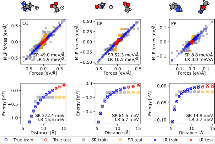
For each class, the upper panel shows a snapshot of the system with the charge states indicated, the middle panel shows the parity plot for the force components, and the lower panel shows the binding energy curve, which is the potential energy difference between the dimer, and two isolated and relaxed monomers. The root mean square errors (RMSE) for the energy and force components of the test sets are shown in the insets.
The goal of this benchmark is to evaluate whether the MLIP models can extrapolate dimer interactions at larger separations based on training data from smaller distances. For each molecular pair, the training set consists of 10 configurations with dimer separation distances between approximately 5 Å and 12 Å, and the test set includes 3 configurations with separations between approximately 12 Å and 15 Å.
For each molecular pair, we trained a short-range (SR) model using CACE with a cutoff rcut = 5 Å, 6 Bessel radial functions, c = 8, \({l}_{\max }=2\), \({\nu }_{\max }=2\), Nembedding = 3, and one message passing layer (T = 1). It should be noted that this setting of the “SR” model already achieves a perceptive field of 10 Å through the message passing layer, which is quite typical for current MPNNs. In comparison, more traditional MLIPs based on local atomic descriptors typically use a cutoff of around 5 or 6 Å, making them even more short-ranged.
In the long-range (LR) model, the short-range component Esr used the same CACE setup, while the long-range component Elr employed a 4-dimensional hidden variable computed from the same CACE B-features and utilized Ewald summation (Eq. (4)) with σ = 1 Å and a k-point cutoff of kc = 2π/3. It is important to fit both energy and forces for these datasets, as fitting only to a few energy values may result in models that accurately predict binding energy but perform poorly on forces.
Figure 1 shows that the LR MLIPs outperform the SR MLIPs in all cases. Furthermore, SR models fail to adequately capture the training data, as indicated by the flattening of the binding curves and the large discrepancies between some predicted and true forces (gray symbols in Fig. 1). The primary limitation of the SR models is that molecules separated by distances beyond the MLIP cutoff exist on independent atomic graphs, rendering the message-passing layers ineffective for communication between the dimers. Direct comparison of the accuracy of the present LR models with the LODE method [7] is challenging, as different training protocols were used in ref. [7], and LODE depends significantly on the choice of the potential exponent p for each dimer class. However, based solely on RMSE values, the LR models presented here appear to be more accurate. For example, in the CC class, the energy RMSE is 15.5 meV, compared to approximately 0.1 eV for LODE with the optimal choice of p.
Example on molten NaCl
Molten bulk sodium chloride (NaCl) presents non-negligible long-range electrostatic interactions. The dataset from ref. 25 contains 1014 structures (80% train and 20% validation) of 64 Na and 64 Cl atoms. Table 1 compares the root-mean-square percentage error (RMSPE) using different methods. rcut = 6 Å were used for all models except for the LODE flexible (7 Å). The CACE-LR models use 6 Bessel radial functions, c = 12, \({l}_{\max }=3\), \({\nu }_{\max }=3\), Nembedding = 3, zero (T = 0) or one message passing layer (T = 1), a 4-dimensional q, σ = 1 Å and a k-point cutoff of kc = 2π/3 in Ewald summation. The details for the other models are in ref. 25. We also trained hybrid models incorporating long-range electrostatics via element-dependent fixed charges on Na and Cl ions, with the remaining energy and forces fitted to short-ranged CACE T = 0 potentials. One model utilized nominal charges of 1e/-1e for Na/Cl ions, while another employed optimized fixed charges of 0.65e/−0.65e for Na/Cl ions.
Table 1 shows that the short-ranged models, including SOAP27,32,35, MACE30T = 0, and CACE T = 0 exhibit the highest errors. The simple baseline model using nominal fixed charges (CACE + fixed q = 1e) performs worse than the short-range models. However, after optimizing the fixed charge values through training, the CACE + fixed q=0.65e model demonstrates improved accuracy. Other long-ranged models, including LODE7,24 with different settings, a density-based long-range model25, and CACE-LR outperform the purely SR methods. MACE30 with message passing (T = 1), especially the one using equivariant features, also achieves accurate results, as message passing increases the effective perceptive field. Overall, CACE-LR models, with and without message passing (T = 0 and T = 1), obtain the best accuracy.
Example of bulk water
As an example application to dipolar fluids, we applied the LES method to a dataset of 1593 liquid water configurations, each containing 64 molecules36. The dataset was calculated using revPBE0-D3 DFT. For the CACE representation, we used a cutoff of rcut = 5.5 Å, 6 Bessel radial functions with c = 12, \({l}_{\max }=3\), \({\nu }_{\max }=3\), Nembedding = 3, and no message passing (T = 0) or one message passing layer (T = 1). For the long-range component, we used a 4-dimensional q, a maximum cutoff of kc = π, and σ = 1 Å in the Ewald summation.
The learning curves in Fig. 2 demonstrate that message passing significantly improves the accuracy of MLIPs, consistent with previous studies19,30. The LR component further reduces the error for both models without a message-passing layer (T = 0) and with a message-passing layer (T = 1). The improvement is particularly notable in the T = 0 scenario. For the T = 1 models, the LR component results in a smaller reduction in errors, probably because the T = 1 SR models already capture atomic interactions up to 11 Å. Nevertheless, the T = 1 LR model demonstrates greater efficiency in learning with fewer data. We also compared the inference speeds of these models during molecular dynamics (MD) simulations, as detailed in the Methods section.
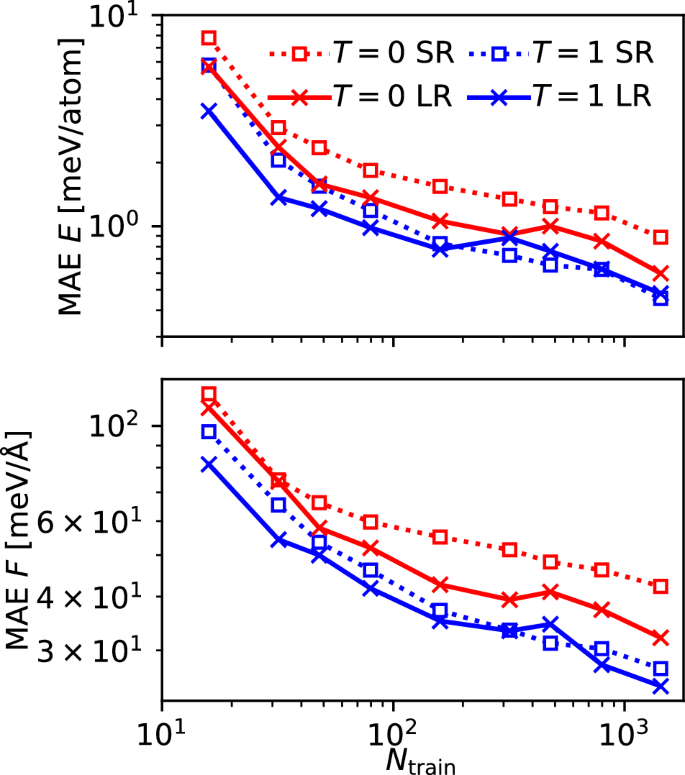
Learning curves of energy (E) and force (F) mean absolute errors (MAEs) on the bulk water dataset36, using short-range (SR) or long-range (LR) models and with or without massage passing layers (T = 0 or T = 1).
To investigate how message passing and long-range interactions affect predicted structural properties, we performed MD simulations of bulk water with a density of 1 g/mL at 300 K using each model. The upper panel of Fig. 3 shows the oxygen-oxygen (O-O) radial distribution function (RDF) computed with different MLIPs. All computed O-O RDFs are indistinguishable and in excellent agreement with the experimental results of the X-ray diffraction measurements37. This suggests that local representations are sufficient to accurately predict the RDFs of bulk liquid water, consistent with previous findings3.
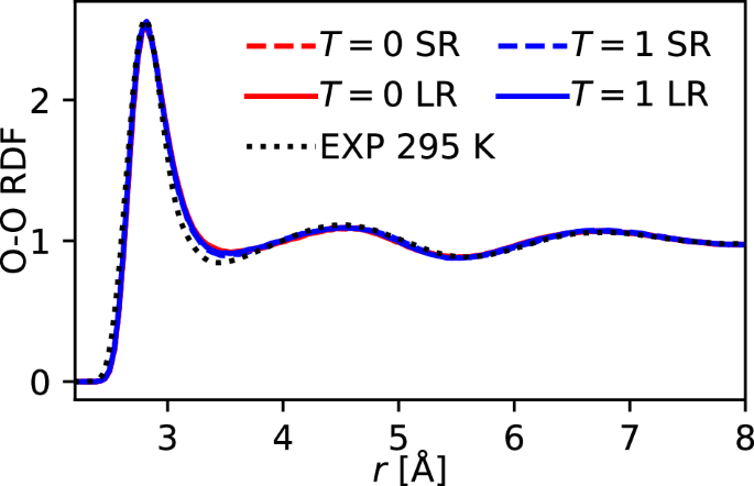
The experimental O-O RDF at ambient conditions was obtained from ref. 37.
We then investigated the effect of long-range interactions on the dielectric properties of water by computing the longitudinal component of the dipole density correlation function6, \(\langle {\widetilde{m}}_{z}^{\star }(k){\widetilde{m}}_{z}(k)\rangle\), where \(\widetilde{m}\) is the Fourier transform of the molecular dipole density and k = kz is along the z-axis. The dipole correlation function at the long-wavelength limit can be used to determine the dielectric constant of water12.
As shown in Fig. 4, while the dipole density correlation functions predicted by different MLIPs are in excellent agreement for most values of k, discrepancies emerge at long wavelengths. Specifically, the results from short-ranged models sharply increase as k → 0. This divergence has also been observed in previous studies comparing the SR and LR models6,12. The divergence of the T = 0 short-ranged MLIP appears at a k value corresponding to a real length scale of approximately 11 Å, while the T = 1 SR model diverges at about 16 Å. Interestingly, these length scales, where divergence occurs, exceed the effective cutoff radius, suggesting that SR MLIPs may partially describe long-range effects beyond their cutoffs in a mean-field manner. When comparing the two SR MLIPs, the message passing layer delays the onset of divergence at small k values but does not eliminate it. In this scenario, only true LR models can adequately describe the dielectric response.
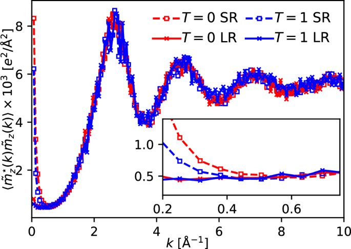
The inset shows a zoom-in of the small k values.
Example on interfacial water
It is widely recognized that short-range MLIPs fall short in describing interfaces4,12. To demonstrate the efficacy of the LES method for interfaces, we used a liquid-water interface dataset from ref. 4, computed with the revPBE-D3 functional. This data set contains approximately 17,500 training configurations, and was used to train a short-ranged DeePMD model17 combined with a long-range electrostatic baseline employing charges taken from an empirical water force field4. From these, we selected a small subset of 500 liquid-vapor interface configurations, each containing 522 water molecules.
We employed the same settings for fitting the MLIPs as used for the bulk water dataset. The learning curves for forces are shown in Fig. 5. The energy errors are very low, reaching less than 0.1 meV/atom in mean absolute error (MAE) for all models using only 50 training configurations. The force errors are also small, ranging from about 14 meV/Å to 27 meV/Å in MAE when trained on 90% of the dataset. The learning behavior is similar to that observed in the bulk water case: both message passing and long-range interactions enhance the accuracy of the MLIPs.
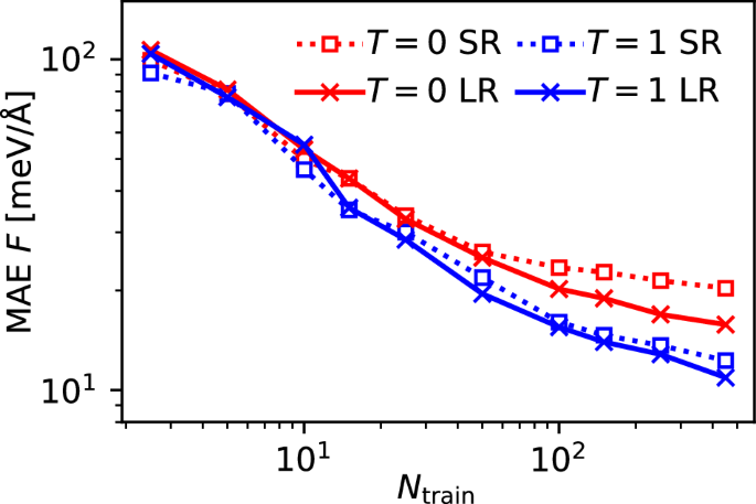
Learning curves on the liquid-vapor water interface dataset4 using the short-range (SR) and long-range (LR) models with no message passing (T = 0) or one message passing layers (T = 1).
For each of the T = 0 SR, T = 0 LR, T = 1 SR, and T = 1 LR models, we trained three MLIPs using different random splits of 90% for training and 10% for testing. We then simulated the liquid-vapor interface at 300 K using both a thinner slab (Fig. 6a) and a thicker slab of about double the thickness (Fig. 6d). The resulting density profiles of the water slabs are shown in Fig. 6b, e. All SR and LR models predict similar density profiles, and for the thinner slab, all models accurately reproduce the density profiles of the reference DFT water data.
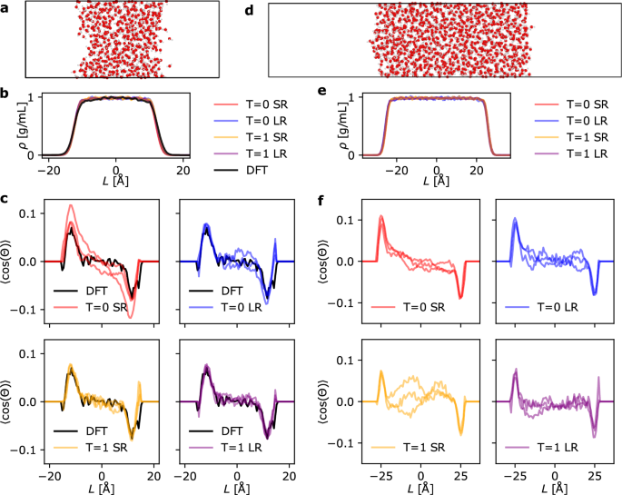
a shows a snapshot of the thinner water slab configuration, b shows the water density profile, and c shows average cosine (c) the average \(\cos (\theta )\) for the angle formed by the water dipole moment and z-axis. DFT results are from ref. 4. d, e and f show the snapshot, the water density, and \(\langle \cos (\theta )\rangle\) for the thicker water slab, respectively.
In addition to density profiles, we evaluated the orientational order profiles, shown in Fig. 6c, f, by computing the angle, θ, between the dipole orientation of water molecules and the z-axis. For each model, the three different fits of MLIPs provide slightly different predictions, and the variances are larger for the SR models compared to the LR models. At the interfaces, water molecules tend to form a dipole layer, which is screened by subsequent layers, ensuring that the bulk does not exhibit net dipole moments4. However, without long-range interactions, this screening effect is not adequately captured, leading to extended dipole ordering into the bulk as seen in the T = 0 SR model. The introduction of message passing (T = 1 SR model) alleviates this issue at least for the thinner slab, but it also introduces an artifact: dipole ordering in the bulk along the opposite direction for the thicker slab. In contrast, on average and with smaller variance between different fits, the LR models recover the correct orientational order profiles, effectively capturing the screening effect and accurately representing the physical polarization behavior at the liquid-vapor interfaces.


