Large-scale discovery, analysis and design of protein energy landscapes

Library design

The initial set of 15,715 domain sequences was organized into five batches and further divided into 18 libraries (mix 1–4, libraries 1 and 4; libraries 7–15; and mutants 2–4): (1) mix 1–4: de novo designed ααα, βαββ and ββαββ sequences²¹; (2) libraries 1 and 4: de novo designed αββα proteins¹¹; (3) libraries 7–14: natural domains from the Pfam database, including LysM, PASTA, WW, SH3, pyrin and cold-shock; (4) library 15: PDB-derived monomeric proteins devoid of cysteine residues and metal cofactors; (5) mutant libraries containing single and double mutants from EEHEE_rd4_0871 and HHH_rd4_0518 low-cooperativity proteins. Sequences were randomly assigned to libraries within each batch, ensuring a minimum mass difference of 50 ppm between nearest-neighbour sequences for mass spectrometry compatibility (except library 15 where two sequences are 36 ppm apart). After SUMO cleavage (see below), all proteins begin with the dipeptide HM (the scar from the NdeI ligation). Some sequences were modified with C-terminal padding (G, S, GG or GS) to optimize mass spacing. All sequences were reverse-translated and codon-optimized for E. coli using DNAworks (v.2.0)⁶⁸. To standardize amplification efficiency, a ‘GGS’ sequence was appended after the stop codon. Oligo libraries encoding the original 15,715 sequences were purchased from Agilent Technologies, while the 280 designed mutations were sourced from Twist Bioscience.

Cloning of Twist oligo libraries into the pGR02 plasmid

Oligo libraries were resuspended and amplified by quantitative PCR (qPCR) for restriction enzyme cloning. A preliminary qPCR run determined optimal amplification cycles, preventing overamplification by terminating reactions at around 50% of maximum fluorescence intensity. Purified qPCR products were digested with XhoI and NdeI and ligated into the pGR02 plasmid, which encodes an N-terminal 10×His-SUMO tag. Ligated constructs were electroporated into 10-β electrocompetent E. coli (New England Biolabs) and recovered in SOC medium at 37 °C for 1 h before plating onto selective MDAG-11 + B1 + kanamycin agar plates⁶⁹. Serial dilutions determined transformation efficiency, and all colonies were pooled to maximize sequence diversity. Plasmid DNA was extracted from pooled cultures using the QIAprep Spin Miniprep Kit (Qiagen).

Library expression and purification

Each library’s plasmid pool (5 μl) was electroporated into 25 μl BL21(DE3) electrocompetent E. coli (Sigma-Aldrich), recovered in SOC medium (1 ml, 37 °C, 1 h), and plated onto selective MDAG-11 + B1 + kanamycin agar plates. Colonies were pooled and used to inoculate 2–4 l of LB broth with 50 μg ml⁻¹ kanamycin. Cultures were grown at 37 °C until an optical density at 600 nm (OD₆₀₀) of 0.6, then induced with 1 mM IPTG and incubated at 16 °C overnight (~16 h). Cells were collected by centrifugation and resuspended in lysis buffer (20 mM Tris, 500 mM NaCl, 30 mM imidazole, 0.25% CHAPS, 1 mg ml⁻¹ lysozyme, 10 U ml⁻¹ Benzonase, 1× Pierce protease inhibitor cocktail, pH 8.0). Sonication (QSonica, 5 min total, 60% amplitude, 1 min on/off cycles) was followed by centrifugation (12,500g, 30 min, 4 °C; repeated at 14,000g for clarification). The soluble fraction was purified through Ni-NTA agarose gravity columns (Qiagen). After washing with buffer (20 mM Tris, 500 mM NaCl, 30 mM imidazole, 0.25% CHAPS, 5% glycerol, pH 8.0), proteins were eluted (20 mM Tris, 300 mM NaCl, 500 mM imidazole, 5% glycerol, pH 8.0). Eluted proteins were dialysed overnight into PBS, and SUMO tags were cleaved using a 1:100 molar ratio of ULP1 (4 °C, ~20 h). A second Ni-NTA purification removed SUMO and ULP1, collecting cleaved proteins in the flow-through. Proteins were concentrated (3 kDa Amicon Ultra filters) and further purified by Superdex 75 10/300 GL size-exclusion chromatography (Cytiva) on the NGC FPLC system (Bio-Rad). The monomeric fractions were pooled, reconcentrated, filtered (0.22 μm Millex-GP filter), flash-frozen in liquid nitrogen and stored at −80 °C until use.

Labelled protein expression and purification for NMR analysis

We selected 13 proteins for individual expression, purification and NMR analysis. The DNA sequences were codon-optimized for E. coli and cloned into pET-28a(+) (thrombin cleavage site) from Twist Biosciences or pET-28a(+)-TEV from GenScript. The plasmids were transformed into chemically competent BL21(DE3) cells. A small starter culture (5 ml) was inoculated in LB Miller broth with 50 μg ml⁻¹ kanamycin and grown overnight at 37 °C, 220 rpm. The starter culture (25 μl) was then diluted into 50 ml of labelled M9 medium (42 mM Na₂HPO₄, 22 mM KH₂PO₄, 8.6 mM NaCl, 8.6 mM 15NH₄Cl (Cambridge Isotope), 11 mM d-glucose (¹³C, Cambridge Isotope), 1 mM MgSO₄, 0.2 mM CaCl₂, 0.15 mM thiamine, 1% (v/v) trace elements (3 mM FeCl₃, 0.37 mM ZnCl₂, 0.074 mM CuCl₂, 0.042 mM CoCl₂·H2O, 0.162 mM H₃BO₃, 6.84 mM MnCl₂·H₂O)) with 50 μg ml⁻¹ kanamycin and grown overnight at 37 °C, 220 rpm. Larger cultures of M9 medium were inoculated with overnight M9 small culture (50 ml per 1 l) and grown at 37 °C, 220 rpm to OD₆₀₀ of around 0.6. Expression was induced with 0.5 mM IPTG, and cells were incubated at 16 °C overnight (around 16–18 h). Cells were collected, resuspended in lysis buffer (20 mM Tris, 500 mM NaCl, 30 mM imidazole, 0.25% CHAPS, pH 8.0, 1 mg ml⁻¹ lysozyme, 10 U ml⁻¹ Benzonase, 1× Pierce protease inhibitor EDTA-free) and lysed by sonication. The lysates were clarified by centrifugation (13,000g, 30 min). Proteins were purified by immobilized metal affinity chromatography (IMAC) using Ni-NTA agarose. The column was washed with buffer (20 mM Tris, 500 mM NaCl, 30 mM imidazole, 0.25% CHAPS, 5% glycerol, pH 8.0), and proteins were eluted in elution buffer (20 mM Tris, 300 mM NaCl, 500 mM imidazole, 5% glycerol, pH 8.0). Eluted proteins were dialysed into buffer (50 mM Tris, 200 mM NaCl, 5% glycerol, pH 8.0) using Pur-A-Lyzer dialysis tubes (Sigma-Aldrich). His-tags were cleaved using either TEV protease (produced in-house, pRK793 plasmid; Addgene, 8827) or thrombin CleanCleave kit (Sigma-Aldrich), depending on the construct. TEV protease was added at a protease:target protein ratio of 1:10 with 0.5 mM DTT and incubated overnight at room temperature. Thrombin cleavage followed the manufacturer’s protocol, incubating overnight at room temperature. A second IMAC Ni-NTA purification was performed to remove the tag and uncleaved protein. Proteins were further purified by size-exclusion chromatography using a Superdex 75 10/300 column in phosphate-buffered saline. Monomeric fractions were identified based on elution profiles of a standard mixture (BSA, ovalbumin, ribonuclease A, aprotinin and vitamin B12), pooled, and concentrated using Amicon Ultra-4 centrifugal filters. The protein concentration was determined using the Pierce BCA assay (Thermo Fisher Scientific).

NMR structure determination

NMR spectra for HHH_rd4_0518, EEHEE_rd4_0871 and EEHEE_rd4_0642 structure calculations were acquired at 288 K on Bruker spectrometers operating at 600 and 800 MHz, equipped with TCI cryoprobes with the protein buffered in 20 mM sodium phosphate (pH 7.5, 150 mM NaCl) at concentrations of 0.5 to 1 mM. Resonance assignments for ¹⁵N/¹³C-labelled proteins were determined using FMCGUI⁷⁰ based on a standard suite of 3D triple- and double-resonance NMR experiments collected as described previously⁷¹. All 3D spectra were acquired with non-uniform sampling in the indirect dimensions and were reconstructed by the multi-dimensional decomposition software qMDD⁷², interfaced with NMRPipe⁷³. Peak picking was performed manually using NMRFAM-Sparky⁷⁴. Torsion angle restraints were derived from TALOS+⁷⁵. Automated NOE assignments and structure calculations were conducted using CYANA (v.2.1)⁷⁶. The best 20 out of 100 CYANA-generated structures were refined with CNSSOLVE⁷⁷ by performing a short restrained molecular dynamics simulation in explicit solvent⁷⁸. The final 20 refined structures comprise the NMR ensemble. Structure quality scores were performed using Procheck analysis⁷⁹ and the PSVS server⁸⁰.

HDX NMR analysis

NMR HDX rates were measured for 13 proteins. A detailed overview of the experimental conditions, including buffer composition, temperature, pH and protein constructs, is provided in Supplementary Fig. 5 and Supplementary Table 1 (dataset 4). Exchange experiments were conducted at 600 MHz by tracking the decay of amide peak intensities in ¹H-¹⁵N HSQC spectra over a 24 h period. Proteins were lyophilized in their respective analysis buffers, and exchange was initiated by dissolving them in an equivalent volume of D₂O. Each HSQC timepoint required approximately 5 min for acquisition, with the first measurement occurring around 5 min after exchange initiation. Peak intensity data were fitted to a single exponential decay, and opening free energies were derived from these rates as described previously^67,81,82.

mHDX-MS analysis

Library samples (0.1–1 mg ml⁻¹) were diluted 1:9 into deuterated buffer (95% D₂O), either 25 mM MES (for pH_read ≈ 6) or 25 mM bicine (for pH_read ≈ 9). At specified incubation times, 95 µl of the exchange solution was mixed with 25 µl of quench buffer (0.5 M Gly–HCl, pH 2.1–2.3). All sample handling was fully automated using a PAL3 LEAP HDxTool: incubation in D₂O buffer took place in a chamber at 20 °C, while quenching was performed in a chamber maintained at 0 °C. All buffers were individually adjusted before the experiment so that final pH_read values were 6.0 ± 0.05 (MES buffer) or 9.0 ± 0.05 (bicine buffer) and quench conditions were pH_read = 2.45 ± 0.05 after diluting with the sample. The quenched samples were then analysed on the Waters Synapt G2-Si Q–TOF mass spectrometer equipped with a Waters HDX Manager. Chromatography separation was performed at 0 °C on a 1 mm × 100 mm BEH C4 column (300 Å, 1.7 µm particles) using a 30 min gradient, with the entire system maintained at 0 °C to minimize back exchange. Each library was measured in two batches—one at pH 6 and one at pH 9—collecting 32 timepoints (log-spaced from 25 s to 24 h) plus three undeuterated replicates distributed throughout the experiment. All MS runs were performed in MS1-only mode at 1 scan per second. Every 10 s, one scan of sodium formate solution was collected for use in post-processing calibration.

The computational pipeline for mHDX-MS

We developed a computational pipeline for mHDX-MS analysis that is organized into two complementary repositories: mhdx_pipeline (available at https://github.com/Rocklin-Lab/mhdx_pipeline), which handles the processing of LC–IMS-MS data (converted from mzML) through protein identification, signal decomposition through tensor factorization and the assembly of time-dependent mass distributions using a path optimization module; and hdxrate_pipeline (available at https://github.com/Rocklin-Lab/hdxrate_pipeline), which applies back-exchange correction, performs rate fitting via Bayesian optimization and converts these rates into opening free energies. These pipelines are implemented using Snakemake^83,84, enabling reproducible, scalable and parallel processing across compute clusters, thereby enhancing workflow efficiency and facilitating easy re-execution of the entire analysis. We also made available mhdx_analysis (https://github.com/Rocklin-Lab/mhdx_analysis) to provide readers with useful code for post processing of mHDX-MS results. Our entire codebase is freely available under CC BY 4.0 license. Below we describe the main components of both pipelines.

Protein identification

We used IMTBX and Grppr to extract the set of protein-like isotopic clusters (ICs) to allow for automated processing of the undeuterated samples⁸⁵. We use the default parameters except that we do not apply automatic mass correction. Calibration was performed as described below. Protein identification is performed solely based on the MS1 intact mass, with our library designed so that each protein exhibits a unique mass (>50 ppm, except library 15, for which two sequences were within 36 ppm). In our pipeline, we have three sequential quality-control steps for protein identification: (1) mass error filtering: proteins are filtered based on their absolute protein monoisotopic mass error <10 ppm of theoretical values; (2) isotopic distribution matching: identified proteins are further filtered based on a dot product of experimental and theoretical isotopic distributions (idotp), with a threshold idotp > 0.98; (3) we also implemented a false-discovery rate (FDR) estimation and control: a target-decoy strategy to estimate and control for FDR. In this strategy, we generate a decoy sequence database that is twice the size of the initial target library. Decoy sequences are sequences randomized within the expected mass range of target sequences (±50 Da) and are designed to be at least 50 ppm apart from their nearest mass neighbour. At this stage, proteins passing the mass error and idotp thresholds often include an expected greater number of target sequences compared to decoy sequences. This prefiltered dataset is then used for FDR estimation. We trained a regularized logistic regression model to discriminate between identifications from the target database and those from the decoy database. We extract 36 features, including charge-based features, ppm deviation, idotp, intensity metrics and retention time (RT) residual errors. RT residual errors are calculated using a linear regression model trained on the target dataset to predict RT based on amino acid composition. The squared difference between the experimental and predicted RT is used as an additional descriptor for our logistic regression model. The trained logistic regression model outputs probabilities for both the target dataset and the held-out decoy set. At each probability threshold, we estimate the FDR as the ratio of decoys to targets above the threshold. For individual identifications, q values are calculated as the proportion of decoys relative to targets observed above the given probability threshold. Proteins are filtered based on a q-value threshold of 0.025, corresponding to an estimated FDR of 2.5%. In this work, steps 1 and 2 were applied as initial filters for downstream analyses, while step 3 served as a post-processing step. The regularized logistic regression model was trained using all library results (excluding mutant libraries) to derive a unified classification model. This model was then applied to mutant libraries, using the probability threshold (P = 0.803) observed to achieve an FDR of 2.5% in the training data.

MS calibration

To ensure mass accuracy during the analysis, we implemented a lockmass calibration strategy using a reference compound. In this work, we used a solution with sodium formate (1:1:18 0.1 M NaOH:10% formic acid:acetonitrile) as a calibrant. In our pipeline, raw MS data files in .mzML format are parsed to extract individual scans and their respective RTs. For each scan, the experimental spectrum is filtered to retain peaks within a predefined mass-to-charge (m/z) tolerance of 100 ppm around theoretical reference masses. Filtered peaks with intensities exceeding 500 are grouped into chromatographic time bins (5 bins across a 30 min runtime). This allows localized analysis of reference peaks to account for time-dependent variations. For each reference m/z value, a Gaussian function is fitted to the experimental peaks in the filtered spectrum. Peaks with residual errors exceeding the defined 100 ppm tolerance or intensities below the threshold are excluded from calibration. For valid peaks, the observed m/z values are matched to the corresponding theoretical values. We build a linear regression curve to map observed m/z values to theoretical reference values. The calibration curve coefficients are stored and applied to correct all experimental m/z values within the dataset either at the stage of protein identification (see the ‘Protein identification’ section) or at the tensor extraction stage (see the ‘Tensor extraction’ section).

Tensor extraction

To isolate individual protein signals from our LC–IMS-MS data, we represented each experiment as a 3D tensor spanning RT, drift time (DT) and m/z dimensions. For each protein and charge state at each timepoint, we extracted a sub-tensor centred on the protein’s observed RT and DT (and window of ±0.4 min for RT, ±6% of DT centre for DT), plus m/z range corresponding to the expected isotopic envelope extended to the maximum possible deuteration. RT and DT centres were empirically defined by averaging what was observed across undeuterated replicates to account for experimental variability. We applied m/z calibration corrections before extracting each sub-tensor to refine mass accuracy according to the strategy described above.

Tensor factorization for signal decomposition

We next performed iterative factorization using a rank-decomposition approach (such as non-negative matrix factorization in multiple dimensions; schematics are provided in Supplementary Fig. 1a)⁸⁶. We smoothed the sub-tensor in the RT and DT dimensions using small Gaussian kernels (σ_RT,σ_DT = (3,1)) to improve the signal-to-noise ratio. Beginning with an initial guess of k = 5 factors, if the minimum correlation across RT, DT or m/z dimensions between any pair of factors exceeded a specified threshold of 0.17, we considered the data over-factorized and reduced k accordingly. This adaptive process continued until factors were sufficiently distinct. If factors were initially sufficiently distinct, we increased k until we observed over-factorization, keeping the previous iteration. Each resulting factor was further filtered by their Gaussian fit quality in RT and DT (R² ≥ 0.90) to ensure that they represented coherent elution or drift profiles. Next, we examined each factor for multiple ICs. We projected each factor’s m/z dimension to create an integrated mass profile, then used a peak-finding algorithm to locate individual clusters. If more than one cluster was detected, we split the factor accordingly, treating each IC as a distinct signal component. This procedure enabled us to separate closely spaced isotopic envelopes and reduce noise-induced over-segmentation, ultimately yielding the collection of signals for downstream analyses.

PO for assembly of time-course mass distributions

After extracting and resolving signals for each protein and timepoint, we assembled a consistent, time-resolved mass profile for each protein by selecting the most plausible IC at each timepoint using the path optimizer (PO) module in our pipeline. The resulting path spans the undeuterated (initial) to increasingly deuterated (late) states. All ICs—regardless of their charge state—are analysed together by converting each m/z signal into a neutral mass representation (that is, baseline-integrated mass distribution). Before path optimization, we derive nine quantitative features for each IC: (1) RT/DT errors: we compute the deviation in each IC’s RT (s) and DT (percentage) relative to the undeuterated reference signal; (2) RT/DT profile similarity: the cross-correlation between each IC’s elution profile (RT or DT) and that of the undeuterated reference quantifies overall shape similarity; (3) peak error: we compare the observed mass to a theoretical isotopic envelope, penalizing large discrepancies from the expected mass; (4) full width at half maximum (FWHM) deviation: we calculate the FWHM difference relative to the undeuterated reference; (5) intensity deviation: each IC’s integrated intensity is compared to the baseline intensity of the undeuterated protein; unusual gains or losses raise suspicion; and (6) neighbour correlation: if a protein exhibits multiple charge states at a given timepoint, we compute a correlation across m/z and RT dimensions to ensure they represent the same underlying species. ICs lacking other charge states are assigned zero correlation. (7) Signal noise estimation: the integrated mass distribution is fitted to a Gaussian, higher noise or incomplete peaks indicate lower quality, and result in higher values.

To reduce the number of low-quality or redundant ICs before optimization, we apply two complementary filtering strategies: (1) user-defined thresholds: each IC is evaluated against empirical cutoffs for multiple features (for example, maximum RT/DT errors, minimum RT/DT cross-correlation, maximum mass error). ICs exceeding these thresholds (or failing to meet minimum criteria) are excluded outright, ensuring that only clusters within typical experimental bounds proceed to the next stage. (2) Weak Pareto dominance: within each timepoint, we compare ICs that have similar baseline-integrated neutral masses. If one IC is strictly worse than another on multiple metrics (for example, higher RT/DT errors, lower RT/DT profile fits, greater peak error), it is Pareto-dominated and removed. This pruning further refines the set of plausible ICs by discarding those demonstrably inferior across key features.

After prefiltering, we create an array of hypothetical deuteration trajectories, each characterized by a starting fractional uptake and a slope parameter in logarithmic space. For each trajectory, our algorithm selects the best undeuterated IC (based on the dot product with the theoretical isotopic distribution, idotp) and next proceeds across subsequent timepoints, selecting the IC of which the baseline-integrated mass is closest to the trajectory’s expected deuteration level. Each of these initial sampled paths undergoes a greedy local refinement search where we iteratively swap out a single IC at a time if a replacement lowers the path score. Specifically, at each timepoint, we consider all ICs and check whether substituting any single IC yields a better overall path. This iterative process continues until no single substitution can further reduce the path score. Each potential time-course path is evaluated using a multidimensional scoring function that sums several penalty terms that capture low data quality or physically implausible behaviour. The physically implausible behaviour is assessed for whether mass addition between consecutive timepoints does not decrease (no negative uptake) and does not change abruptly (average deuterium uptake does not become faster with time). From the final paths, after the greedy swaps, we choose the one with the lowest score as the winner. This path represents the most coherent set of ICs from undeuterated through late timepoints.

Before downstream analysis, the pipeline runs the PO module in a temporary mode, generating a set of best-fit paths from all proteins to collect statistics (for example, typical RT/DT error, baseline mass deviations). These statistics are aggregated to define empirical thresholds (for example, 2 s.d. above/below the mean) that exclude outlier signals. For each protein, the pipeline then repeats path optimization as described above with these thresholds in non-temporary mode, ignoring candidate clusters failing the newly established criteria. This two-stage approach filters low-quality clusters and yields more robust final time courses. Final paths with a path score (PO total score) of lower than 50 were selected for rate fitting.

Back-exchange correction in mHDX-MS

In HDX-MS, deuterated residues can back exchange to hydrogen during the quenching step and during LC (performed in a non-deuterated buffer). The level of back exchange varies from protein to protein (affecting all measurements of the same protein in a uniform way) and also varies timepoint to timepoint based on small differences in conditions (affecting all proteins in the sample in a uniform way). We correct all measurements using both timepoint-specific and protein-specific corrections to determine the original level of deuteration before any back exchange. Although different residues in each protein may back exchange at different rates, our model assumes a single overall back-exchange percentage for all residues in a given protein at a given timepoint (equation (3)).

Protein-specific back-exchange correction

We determine the percentage of back exchange for each protein based on the deuteration level observed in the longest timepoint (typically 24 h) when the total deuteration is no longer changing (that is, the protein achieved full deuteration and any missing deuteriums are the result of back exchange). Back- exchange percentages are computed separately for pH_read 6 experiments and pH_read 9 experiments for each protein. For proteins that do not reach full deuteration in pH_read 6 experiments, we estimate their pH_read 6 back exchange level based on an empirical linear correlation between back exchange measured at pH 6 (for other, fully deuterated proteins) and back exchange measured at pH_read 9 (for those same proteins; Extended Data Fig. 1a). Overall, protein-specific back exchange varied from 6 to 45%.

Timepoint-specific back-exchange correction

We identify fully deuterated proteins by checking whether their final five timepoints show ≤1 Da variation in mass (Extended Data Fig. 1b). Next, we check which subset of proteins is fully deuterated in the preceding timepoints by checking whether their centroid masses remain within 6% of that final mass. Owing to the diverse stabilities in our samples, there is typically a subset of unstable proteins that rapidly reach full exchange, serving as internal controls for timepoint-specific back exchange across all timepoints. If fewer than five such proteins are found at a given timepoint, we apply the average back exchange computed from later timepoints where enough fully deuterated proteins were found. The timepoint-specific back exchange correction (which varied from −5% to +4% across all timepoints) is added to each protein’s back-exchange value to determine backexchange(s,t) in equation (3).

Inferring exchange rates from isotopic distributions

We sample a set of exchange rates k_HX (one rate per exchangeable residue) to obtain the posterior rate distribution that is consistent with the observed isotopic envelopes according to the model described in equations (3) and (4). The N-terminal two residues are excluded because these fully back exchange. For domains for which we combine data from pH_read 6 and pH_read 9, we also sample the time scaling factor which determines ‘effective pH_read 6 measurement times’ for all pH_read 9 measurements (Extended Data Fig. 1c–f). This allows for small deviations from a theoretical factor of 10³ due to pH-dependent changes in protein dynamics or charge effects on k_chem.

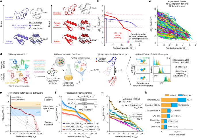
The inputs to the model are the experimentally measured integrated mass distributions at each timepoint (non-zero intensity only), the corresponding timepoints, the theoretical isotopic distribution in the undeuterated state⁸⁷, the estimated level of back exchange at each timepoint and the fraction of D₂O in the exchange buffer. Next, we use Bayesian inference (through no-U-turn sampling (NUTS), as implemented in the numpyro package⁸⁸) to infer the set of amide exchange rates ln(k_HX). We define a hierarchical prior that first samples a slowest rate from a truncated normal centred near e⁻⁷ s⁻¹ (with scale e¹⁰ and bounded below e⁻¹⁵), then linearly spaces a set of N log-rates from this slowest rate up to ln(e¹⁰). Each of the N log-rates is assigned a broad normal prior distribution (σ = 5), reflecting minimal prior knowledge (Fig. 1e). For each proposed set of rates, we compute a Poisson-binomial^89,90 distribution of exchanges—adjusted by the inferred back exchange and deuterium fraction (equation (3))—to yield a convolved theoretical integrated mass envelope per timepoint. Discrepancies between these theoretical envelopes and the measured intensities are captured by a Gaussian distribution with a global noise parameter (drawn from an exponential prior, σ = 1). We run the Markov chain Monte Carlo algorithm with four parallel chains, using 100 warm-up iterations and 250 posterior draws in each chain. After sampling, we discard any problematic chains (for example, poor R-hat or chain-specific r.m.s.e.) and re-run if necessary. Finally, samples from all chains are combined, and each sample’s posterior rate distribution is sorted from slowest to fastest, yielding posterior distributions for each ith slowest rate (with i ranging from 1 to N) as shown in Fig. 1e.

Chemical intrinsic rate approximation in mHDX-MS analysis

To convert our Bayesian-inferred exchange rates k_HX,i into residue opening free energies ΔG_open,i, we must know each site’s intrinsic rate k_chem,i (equation (2)). However, each residue has a unique k_chem,i based on its local sequence context^67,91, and our data do not reveal which measured rate is associated with which residue’s k_chem. A straightforward approximation is simply to use the median (or mean) value among the intrinsic rates. To improve on this approximation, we examined the empirical relationship between k_chem,i and k_HX,i using site-resolved HDX NMR data on 11 proteins (all from Supplementary Fig. 5, except for double mutants HHH_rd4_0518_R35D_G45L and EEHEE_rd4_0871_K31L_E36V). We found a weak but significant trend across nearly all proteins whereby residues with slower k_HX,i also had slower k_chem,i (Supplementary Fig. 2a). We incorporated this trend into our estimation of k_chem,i using a simple scaling factor between normalized k_HX,i and normalized k_chem,i:

where median(log k_chem), z-score(log k_HX,i) and std(log k_chem) are computed separately for each protein, and a universal scaling factor α is used for all proteins. As a result, a residue with the average log k_HX,i for its protein (that is, z-score = 0) will be analysed using that protein’s median k_chem,i, and faster or slower residues will be analysed using faster or slower k_chem,i based on the scaling factor α. Here, we used a scaling factor α = 0.38, which nearly minimizes the error between our inferred ΔG_open distributions and the ΔG_open distributions from NMR across all 11 proteins (this was computed using a smaller set of NMR proteins than our final set). This adjustment yields ΔG_open distributions that are more accurate than assuming the median k_chem for all positions (Supplementary Fig. 2b).

Net charge correction to all ΔG
_open

To account for electrostatic effects on hydrogen exchange rates, we applied a correction to the estimated ΔG_open values based on the estimated net charge of each protein at pH 6 (as computed by the ProtParam module within the Biopython package^92,93). It has been shown that negatively charged proteins have slower k_chem due to decreased local concentration of the hydroxide catalyst, and vice versa^94,95, although these corrections are not explicitly considered in the exchange framework of ref. ⁴⁰. Our data reproduced this electrostatic dependency. To empirically correct for this effect, we derived a linear adjustment that removes the dependency between net charge and ΔG_unfold. For proteins with ΔG_unfold > 4 kcal mol⁻¹, we found the nearly optimal correction coefficient of 0.12 kcal mol⁻¹ per unit charge, which was then applied to all ΔG_open,i values.

ΔG
_unfold calculation

We derive ΔG_unfold as the average across the five more stable residues (averaging across 1–6 residues leads to highly correlated ΔG_unfold estimates; Supplementary Fig. 3a). When deriving ΔG_unfold, we did not account for the contribution of the unfolded state cis–trans isomerization to the measured ΔG_unfold^39,40. Thus, all ΔG_unfold measurements are in reference to an unfolded state in which prolines have their native-state isomerization state, rather than a fully equilibrated unfolded state. However, analysis of proline isomerization states in AlphaFold 2 models (Supplementary Fig. 3b) indicates that cis-prolines are predominantly present in PASTA domains, with minimal occurrence in other protein families analysed (Supplementary Table 1 (dataset 3)). Thus, potential biases due to cis-prolines are largely confined to PASTA and do not substantially affect the other protein families examined. We also did not correct results for the small effects of trans-prolines.

Detecting and filtering EX1 behaviour

Our pipeline is primarily designed for unimodal, EX2-like exchange profiles. It attempts to split multimodal or poorly fitted peaks into separate unimodal peaks, which is not ideal for analysing EX1 kinetics. We therefore do not recommend using this code in its current form to analyse EX1 data. Nonetheless, we implemented an automated procedure to identify and exclude these potential EX1-type profiles from our dataset. Under EX1 kinetics, backbone amides often exhibit an abrupt shift in their isotopic distribution, leading to characteristic anomalies in the experimental and fitted exchange profiles. (1) Width criterion: for each timepoint, we compared the observed isotopic distribution width to the width of the theoretical distribution from our EX2-only fit. We then computed the ratio of these widths across the exchange progress—specifically focusing on timepoints at which the majority of amides (80–90%) had undergone exchange. Samples were flagged as potential EX1 if two conditions were met: (1) the average width ratio in that progress window exceeded 1.25; and (2) the maximum ratio was greater than 1.35. Any domain meeting both thresholds at either pH 6 or pH 9 was classified as ex1_width_criteria. (2) Jump criterion: to capture large, discrete transitions in the exchange profiles, we tracked the difference between the centroid of the fitted distribution (EX2 assumption) and the maximum peak of the observed distribution over time. An exchange profile was labelled as ex1_jump_criteria if it displayed a shift exceeding a predefined range (from less than −2 Da to more than +2 Da) coupled with the transition happening below 90% overall exchange. These constraints were set to identify ‘jumps’ characteristic of EX1-like coordinated exchange rather than the smoother transitions expected under EX2 kinetics. Schematics on each criteria are provided in Extended Data Fig. 2a,b.

Determining full deuteration and protein classification in mHDX-MS

For protein classification, we defined full deuteration as a delta mass of less than 2 Da between the back-exchange-corrected centroid masses measured at the last and fifth-to-last timepoints. Based on this criterion, our data are classified into four groups: (1) unmeasurable proteins, for which full deuteration occurs too early for accurate exchange rate modelling. We also classify a unmeasurable protein if any of following conditions are met: slowest rate constant greater than 10⁻⁴ s⁻¹, ΔG_unfold value is lower than 2 kcal mol⁻¹ or fewer than 20% of residues present measurable exchange rates (k_HX < 10^−3.45 s⁻¹); (2) proteins that achieve full deuteration in the pH 6 experiment; (3) proteins that only reach full deuteration in the pH 9 experiment—requiring the integration of data from both pH 6 and pH 9; and (4) proteins that do not reach full deuteration even in the pH 9 experiment. Proteins belonging to groups (2) and (3) are subsequently referred to as measurably stable.

Filtering low-quality data

To maximize the reliability of our mHDX-MS measurements, we applied a series of filtering criteria (Supplementary Fig. 13). First, low-quality identifications were removed based on mass error (>10 ppm), isotopic distribution matching (idotp < 0.98) and q values (>0.025), and paths with a PO score above 50 were excluded (or above 40 for HHH_rd4_0518 and EEHEE_rd4_0871 mutants) (Supplementary Table 1 (dataset 1)). For all proteins that reach full deuteration, we require overall back exchange to remain below 45% (we do not consider back exchange for proteins in group 4 that do not reach full deuteration). For proteins fully deuterated under both conditions, we required that the back-exchange difference between pH 6 and pH 9 be less than 10%. Moreover, we assessed the consistency between the experimental and theoretical mass distributions (from the inferred rate constants) by requiring that 90% of timepoints have an r.m.s.e. lower than 0.3 normalized units (mass distributions are normalized so that the most intense isotopic peak has an intensity of one unit). This filtered dataset is available as Supplementary Table 1 (dataset 2). Finally, for each protein, the mass distribution path with the lowest PO score was selected as the representative opening energy distribution, and proteins exhibiting EX1 kinetics (Extended Data Fig. 2), unmeasurable protection or incomplete deuteration at pH 9 (Extended Data Fig. 5) were excluded from the measurably stable dataset (Supplementary Table 1 (dataset 3).

Protein structure prediction

We predict the 3D structures of the proteins from their amino acid sequences using AlphaFold 2⁵⁶. The protein sequences, provided in FASTA format, were used as input to the ColabFold implementation of AlphaFold 2⁹⁶, which was run on Quest high performance computing facility at Northwestern University. The pipeline generated five models for each sequence, and the best-scoring model, based on the predicted pLDDT, was refined using amber. The best AlphaFold model for each sequence was further refined using the Rosetta Relax protocol⁹⁷. This process aimed to optimize the predicted structures by minimizing their energy. When not explicitly mentioned otherwise, the relaxed structure was selected for downstream analysis (Supplementary Table 1 (dataset 9)).

Deriving normalized cooperativity and family-normalized cooperativity

We first computed each protein’s average opening free energy (ΔG_avg) as the average of all ΔG_open values, with unmeasurably fast residues set to a lower bound of 0 kcal mol⁻¹. Here, ΔG_avg serves as a simplified proxy for the energies of partially open states on the energy landscape. We then built an empirical model of the typical average opening energy (ΔG_avg,expected) for a given domain based on its global stability (ΔG_unfold), its fraction of exchangeable backbone amides that donate hydrogen bonds (fxn_hb) and its net charge (netq). In our Bayesian regression model, we define the expected average free energy as

where the parameters a, b, c, d and e are sampled from non-informative priors (specifically, a distributed as (∼) normal(1, 3), b ∼ normal(0, 5), e ∼ normal(–1, 3), log(c) ∼ normal(–0.3, 2) with c = exp(log(c)) and d ∼ normal(–0.3, 2) with d = exp(log(d))), and the observation noise is modelled with σ ∼ exponential(1). We run Markov chain Monte Carlo using NUTS (as implemented in numpyro⁸⁸) with 1,000 warm-up iterations and 1,000 samples to obtain the posterior distribution of these parameters. We then used the mean values of the posterior distributions for the parameters a–e (Supplementary Table 2) to compute ΔG_avg,expected for each domain. Finally, we define normalized cooperativity as the z score of the residual between each domain’s experimental ΔG_avg and its predicted value, ΔG_avg,expected:

The hydrogen bonding fraction fxn_hb is defined as the fraction of backbone amides that donate hydrogen bonds to any acceptor (sidechain or backbone) in the molecule. The first two residues (the N terminus and the first amide) are excluded from both the numerator and the denominator because these residues fully back exchange during HDX-MS. Hydrogen bonds are determined using the Rosetta model^55,98 based on AlphaFold 2 structural models that are subsequently relaxed with Rosetta. We call these predicted structures reference structures.

These reference structures are critical for the calculation of normalized cooperativity because they define our expectation for how many protected residues should be observed in a fully cooperative domain. Even if a domain’s native structure under our experimental conditions differs from the reference structure (which may occur because the reference structures are only computational predictions), normalized cooperativity is still computed based on the number of hydrogen bonds in the reference structure. In an extreme case, a protein might be substantially unfolded under our experimental conditions compared with the reference structure. For example, consider a protein with two subdomains where both are folded in the reference structure but only one subdomain is stable under our experimental conditions. Here, ‘cooperativity’ could be interpreted in different ways. If we only consider the fraction of the structure that is stably folded under our experimental conditions, this subdomain might behave in a perfectly two-state manner and be considered highly cooperative. However, the domain as a whole (including both subdomains) is not cooperative because one subdomain can unfold while the other remains folded. Our analysis (based on the reference structure) considers the domain as a whole. In this scenario, ΔG_avg will be low, because the residues in the unfolded subdomain (with low ΔG_open) are included in the average. ΔG_avg,expected will be much higher, because ΔG_avg,expected is computed assuming a larger number of protected residues than are experimentally observed. The result is a low normalized cooperativity, indicating that the full domain (according to the reference structure) is relatively low cooperativity compared to other domains with similar stability in our dataset.

We also include a linear correction for net charge (netq) in the calculation of ΔG_avg,expected. As discussed in the ‘Net charge correction to all ΔG_open’ section, negatively charged proteins tend to exhibit slower k_chem. As a result, negatively charged proteins tend to have a larger fraction of measurably stable residues compared to positively charged proteins (exchange is uniformly slower in negatively charged proteins regardless of conformational stability, so more residues can be measured). Although we correct for this bias by applying a charge correction to all ΔG_open measurements, there is still an uncorrected bias on the number of measurable residues. In fitting k_HX, we use a prior distribution on k_HX that assumes that most residues are very unstable until they are shown to be stable in the data (Fig. 1e). As a result, the inferred k_HX (and ΔG_open) end up being very different for residues that are barely slow enough to be measurable and residues that are barely too fast to be measured. Residues that are just barely measurable end up with ΔG_open of around 2 kcal mol⁻¹, compared with residues that are slightly too fast to be measured, which often have inferred ΔG_open much lower than 0 kcal mol⁻¹ (Fig. 1e). These very low opening energies are set to the lower boundary of ΔG_open = 0 kcal mol⁻¹ when calculating ΔG_avg. As a result, the bias towards more measurable residues in negatively charged proteins ends up biasing ΔG_avg. Including netq in ΔG_avg,expected mitigates this bias to enable a more fair comparison of normalized cooperativity in negatively and positively charged proteins.

We derived two distinct cooperativity metrics. The normalized cooperativity metric is obtained by fitting the model to the entire dataset, while the family-normalized cooperativity metric is derived by fitting the model separately within each protein family (using only families with more than 50 examples in the measurably stable category). For both metrics, we report their normalized versions—computed by subtracting the mean and dividing by the s.d. of the residuals—yielding the normalized cooperativity and family-normalized cooperativity, respectively. A Jupyter Notebook for modelling cooperativity from new data, along with a script to derive cooperativity using our precomputed metrics, are available at GitHub (https://github.com/Rocklin-Lab/mhdx_analysis).

PCA of opening energy profiles

PCA was applied to opening free-energy profiles derived from mHDX-MS measurements for proteins in Dataset_3_MeasurablyStable (3,590 proteins; Supplementary Table 1). For each protein, the opening energy distribution was represented as a one-dimensional vector and zero-padded to the maximum profile length across the dataset before PCA. No additional normalization for protein length, hydrogen-bonding or net charge was applied. PCA was performed either globally across all proteins or separately within individual protein families. For family-specific analyses, PCA was applied independently to proteins belonging to each family. Principal component scores were then correlated with global folding free energy (ΔG_unfold) and family-normalized cooperativity using PCCs.

Reproducibility of opening energy distributions in mHDX-MS

Starting from the filtered dataset (Supplementary Table 1 (dataset 2)), we assessed the reproducibility of measured opening energy distributions across independent mHDX-MS experiments. First, for proteins analysed in multiple libraries, if a protein was represented by more than one opening energy distribution within a given library, we selected the path with the lowest PO score as the representative for that library. Across all libraries, 127 opening energy distribution replicates were identified for 36 different proteins. For each protein, the replicate with the lowest PO score was designated as the reference distribution, and the MAD was computed between the reference and every other replicate for that protein in a different library, considering only the measurable opening energies (that is, excluding energies derived from rates outside the dynamic range). This MAD is shown in Fig. 1f.

We further observed that some proteins were detected at multiple RTs within a single experiment. To evaluate the reproducibility in this context, we started with the opening energy distribution corresponding to the lowest PO score as the reference. We then iteratively added additional distributions only if they were acquired at RTs at least 2 min apart from any previously selected distribution—thereby ensuring that the additional replicates reflected genuine distinct chromatographic events rather than minor experimental variability. Under these criteria, 180 proteins exhibited multiple distinct RT replicates (Supplementary Fig. 14a). Across these replicates, both the MAD for global stability (ΔG_unfold) and the MAD computed over all measurable ΔG_open values were less than 0.5 kcal mol⁻¹ (Supplementary Fig. 14b–d).

Comparison between mHDX-MS and HDX NMR

We compared exchange rate and opening energy measurements obtained from HDX NMR with those derived from mHDX-MS. For the rate comparison, each HDX NMR log-rate was compared to a simulated mHDX-MS log-rate, which was derived by adjusting the measured mHDX-MS rates by the ratio of the median k_chem values between the two conditions. The overall agreement between the two methods was quantified by computing r.m.s.e. across all 511 k_HX measurements collected from 13 proteins in multiple HDX NMR conditions (Supplementary Fig. 5). For the opening energy distributions, each construct’s sorted average ΔG_open (averaged over conditions when multiple HDX NMR conditions were available for the same residue) was compared to the corresponding distribution from mHDX-MS. In cases in which the two distributions differed in length, both distributions were truncated to the length of the shorter distribution. We then computed a single overall r.m.s.e. across all 323 ΔG_open measurements from the 13 proteins.

Feature extraction

Our feature extraction pipeline leverages both interpretable features and PLM embeddings. For the interpretable features, we computed a comprehensive set of predictors that include sequence-based descriptors generated with iFeature⁹⁹ (for example, amino acid composition, grouped amino acid composition and composition–transition–distribution metrics), disorder predictors (ADOPT⁵⁷ and flDPnn¹⁰⁰) and structure-based features derived from AlphaFold2/Rosetta-relaxed models. These structure-based features encompass pLDDT scores from AlphaFold2, a set of Rosetta-based features extensively described previously²¹, solvent accessibility¹⁰¹, as well as custom-derived metrics such as side-chain contact scores, burial scores, hydrogen-bond metrics and an expanded set of secondary structural element-specific descriptors (for example, maximum hydrophobicity of helix-1, average pLDDT of helix-2). A complete set of scripts for computing these features is available at GitHub (https://github.com/Rocklin-Lab/mhdx_analysis/tree/main/scripts/feature_extraction). In total, we extracted 2,800 features common across folds and an additional 2,000–3,700 topology-specific features. Moreover, we extracted embeddings from PLMs—ESM2 (650 million parameters)¹⁰², Unirep¹⁰³ and SaProt¹⁰⁴—to capture contextual sequence information. For ESM2, we averaged the representations from layers 33–36 and flattened the result into an array of 2,560 features per protein sequence, while Unirep and SaProt yielded 1,900 and 1,280 features, respectively.

Feature correlation analysis

PCCs were computed for all derived sequence and structural features with target variables, global stability (ΔG_unfold), normalized cooperativity and family-normalized cooperativity within each protein topology. PCCs were computed using the pearsonr function from SciPy Stats. Bootstrapping was performed with 1,000 resamples to generate the 95% CI for PCCs. 10,000 random permutations of global stability (dg_mean), normalized cooperativity (normalized_cooperativity_model_global) and family-normalized cooperativity (normalized_cooperativity_pf) were generated for the HHH and EEHEE topologies. PCCs were calculated for each random permutation of the target variables with the derived sequence and structural features. The mean and 95% CIs were calculated from the distribution of PCCs of the random permutations with each feature and compared to the experimentally calculated PCC.

Training of machine learning models

We implemented a machine learning pipeline to predict key protein properties—ΔG_unfold and family-normalized cooperativity—using regularized linear models (LassoCV and RidgeCV). We independently evaluated features derived from PLM embeddings (ESM-2, SaProt, Unirep) alongside interpretable features. Our pipeline systematically tests 20 model variations per feature set, comparing models that use the original features to those employing expanded features (including square, inverse and logarithmic transformations), and optionally applying Pearson correlation filtering at thresholds of 5%, 10%, 25% and 50% to remove weakly correlated features. Model training was performed using fivefold cross-validation across three independent random splits. To ensure reproducibility and biological relevance, we applied dynamic clustering with MMseqs2¹⁰⁵ to group similar sequences. For each protein family, sequences were iteratively clustered using a range of minimum sequence identity thresholds (from 0.1 to 0.75), with clustering halted when the largest cluster dropped below 10% of the total sequence count, resulting in final thresholds of between 0.45 and 0.70 across families. These sequence clusters were then randomly assigned to the five folds, ensuring that each fold was as distinct as possible while maintaining balanced representation across protein families (PFs).

By contrast, a first-generation set of models was trained on an earlier version of the dataset where PLM embeddings were derived from ProteinMPNN¹⁰⁶, ESM Inverse Folding 1 (ESM_IF1)¹⁰⁷, Tranception¹⁰⁸, ESM2 (with both 650 million and 3 billion parameters)¹⁰², and hybrid models combining ESM2 with ESM_IF1. For these first-generation models, sequences were assigned randomly to five folds without applying identity-based clustering. Despite this difference in preprocessing, the overall training strategy—using fivefold cross-validation across three independent random splits—remained consistent across both approaches.

In both cases, global models were trained on the full dataset and evaluated on individual PFs, while family-specific models were developed for PFs with more than 200 examples. Model performance was assessed using the R² score aggregated across held-out sets, and final model selection was based on the highest mean R² across the three splits to maximize generalization.

Reporting summary

Further information on research design is available in the Nature Portfolio Reporting Summary linked to this article.